5.6 Joining Data Sets with dplyr
Combining data from multiple sources is a common BI task. dplyr provides join functions for every scenario:
inner_join(): Rows with matching values in both datasets.left_join(): All rows from the left dataset, with matches from the right.right_join(): All rows from the right dataset, with matches from the left.full_join(): All rows from both datasets, with matches where available.semi_join(): Rows from the left dataset that have a match in the right, but only left columns.anti_join(): Rows from the left dataset that have no match in the right.
5.6.1 Preparing Sample Data Frames
We set up two overlapping subsets of mtcars to demonstrate each join type:
mtcars1 <- mtcars[1:15, c("mpg", "cyl", "disp", "hp")]
mtcars1$car_model <- rownames(mtcars[1:15, ])
head(mtcars1)
5.6.1.1 mtcars2 DataFrame
This data frame will contain a different subset of columns, namely gear and carb, along with the car_model column. It will include some car models not present in mtcars1 and exclude others that are, to demonstrate various join behaviors.
mtcars2 <- mtcars[10:25, c("gear", "carb")]
mtcars2$car_model <- rownames(mtcars[10:25, ])
head(mtcars2)
With these sample data frames, we can explore how different dplyr join functions operate.
5.6.2 inner_join()
Purpose: Merges rows with matching values in both tables, providing a dataset that includes only the rows common to both tables.
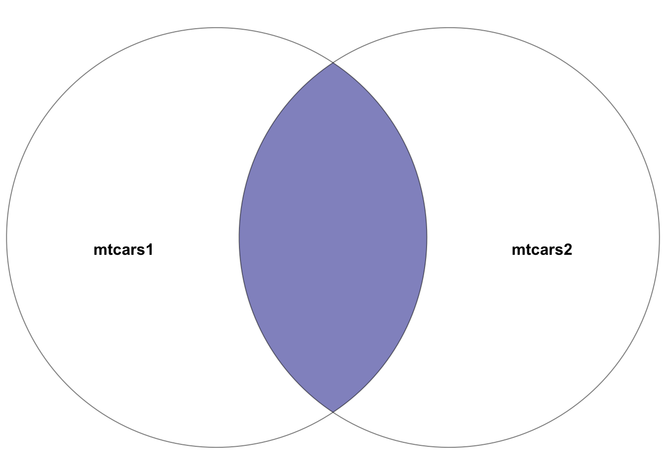
Figure 5.1: Venn diagram showcasing the inner join between the two datasets: mtcars1 and mtcars2. The highlighted section depicts the result of the inner join–the intersection of the two datasets. In other words, the rows with matching entries in the key columns of both datasets
Example:
# Inner join between mtcars1 and mtcars2 on car_model
joined_data_inner <- inner_join(mtcars1, mtcars2, by = "car_model")
head(joined_data_inner)
This join results in a dataset containing cars present in both mtcars1 and mtcars2, with all columns from both datasets included for the matching rows.
5.6.3 left_join()
Purpose: Returns all rows from the left table (first specified), along with the matching rows from the right table. Rows in the left table without matches in the right table will have NA in the columns from the right table.
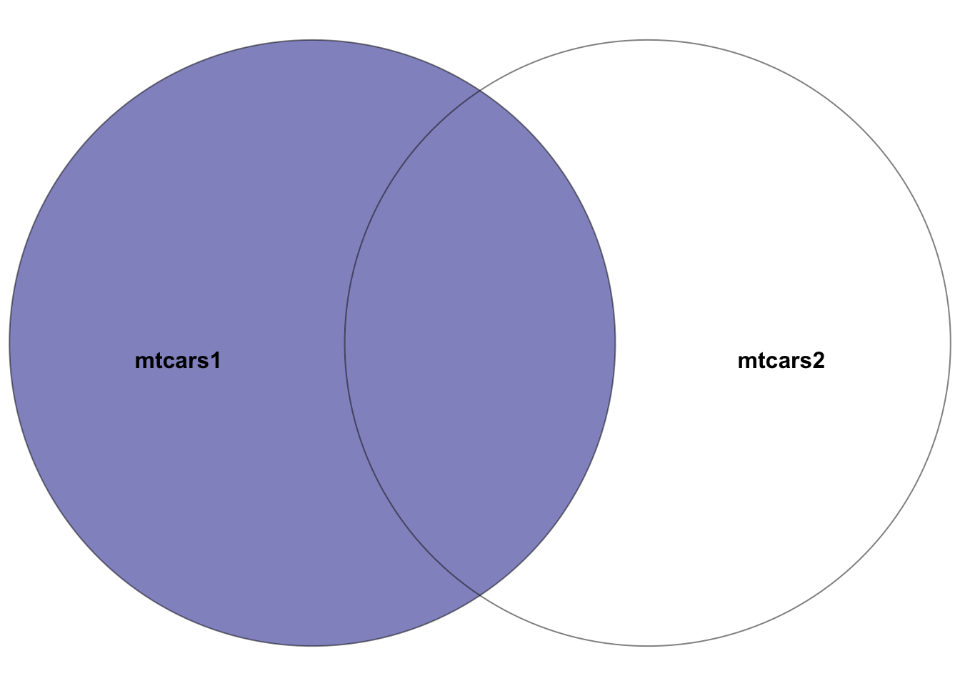
Figure 5.2: Venn diagram showcasing the left join between the two datasets: mtcars1 and mtcars2, where the left dataset is mtcars1. The highlighted section depicts the result of the left join–all rows in the left dataset mtcars1 plus the intersection of the two datasets. In other words, the rows with matching entries in the key columns of both datasets
Example:
# Left join mtcars1 with mtcars2 on car_model
joined_data_left <- left_join(mtcars1, mtcars2, by = "car_model")
head(joined_data_left)
This join produces a dataset with all cars from mtcars1, supplemented with gear and carb data from mtcars2 where available.
5.6.4 right_join()
Purpose: Returns all rows from the right table, with matching rows from the left table. Rows in the right table without matches in the left table will have NA in the columns from the left table.
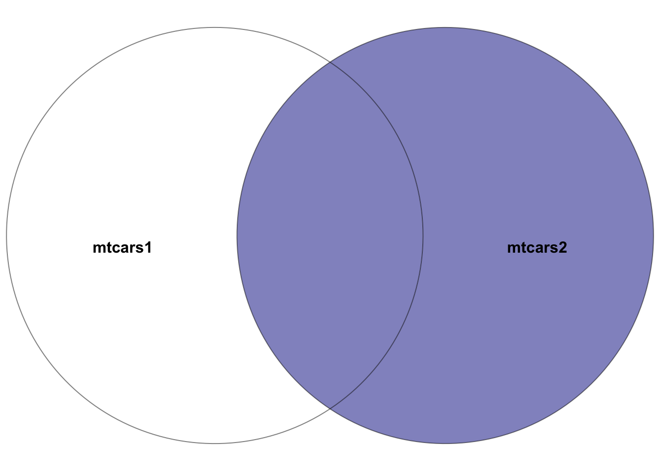
Figure 5.3: Venn diagram showcasing the right join between the two datasets: mtcars1 and mtcars2, where the right dataset is mtcars2. The highlighted section depicts the result of the right join–all rows in the right dataset mtcars2 plus the intersection of the two datasets. In other words, the rows with matching entries in the key columns of both datasets
Example:
# Right join mtcars1 with mtcars2 on car_model
joined_data_right <- right_join(mtcars1, mtcars2, by = "car_model")
head(joined_data_right)
This join yields a dataset containing all cars from mtcars2, with mpg, cyl, disp, and hp data from mtcars1 where matches are found.
5.6.5 full_join()
Purpose: Combines all rows from both tables, with matches where available. Rows without matches in the opposite table will have NA in the corresponding columns.
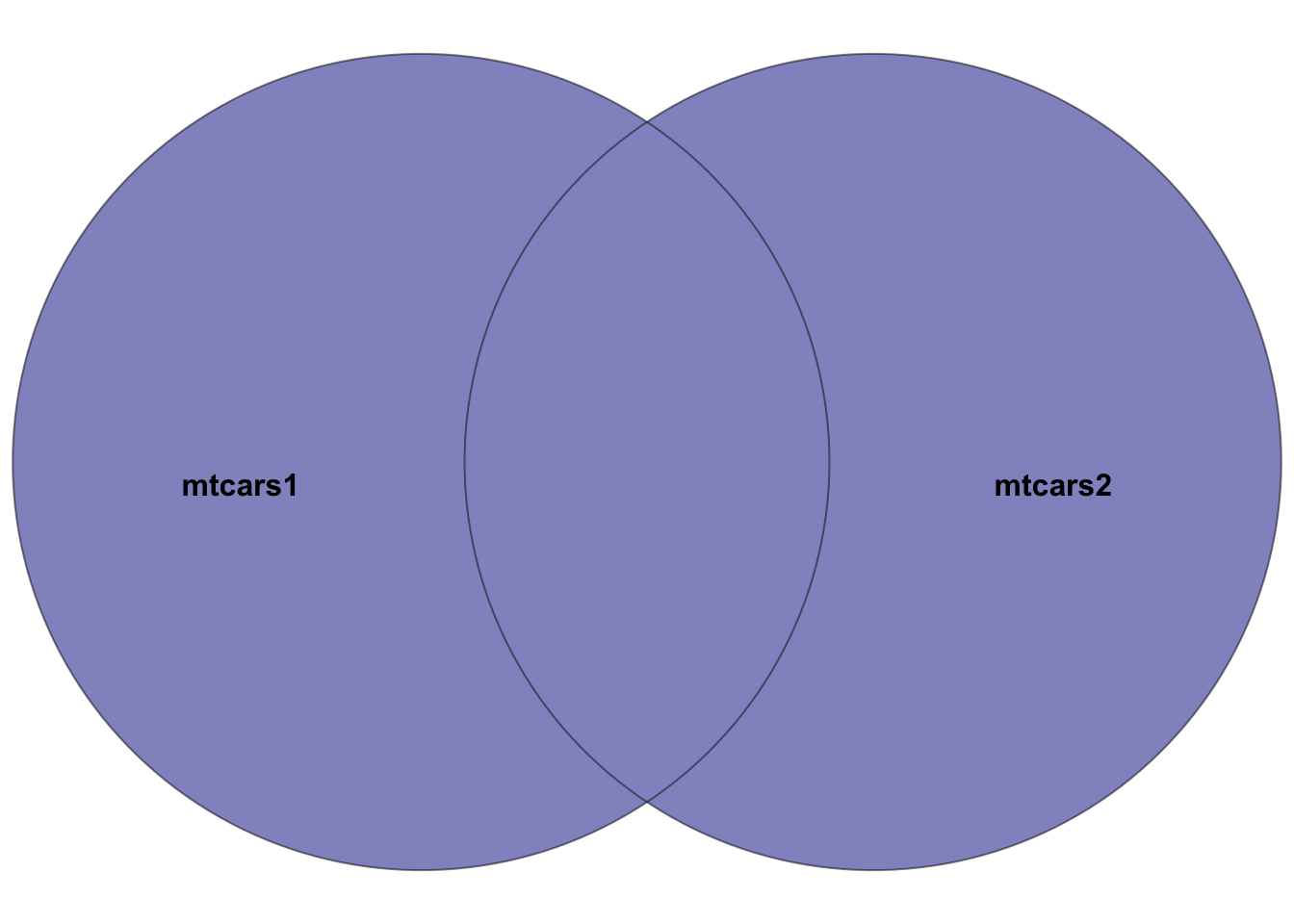
Figure 5.4: Venn diagram showcasing the full join between the two datasets: mtcars1 and mtcars2. The highlighted section depicts the result of the full join–all rows in both datasets. Rows in the intersection of the two datasets will have entries in all columns. Rows not in both datasets will have NA’s in missing columns.
Example:
# Full join between mtcars1 and mtcars2 on car_model
joined_data_full <- full_join(mtcars1, mtcars2, by = "car_model")
head(joined_data_full)
This join results in a dataset that includes all cars from both mtcars1 and mtcars2, ensuring no data is lost, and filling missing values with NA.
5.6.6 semi_join()
Purpose: Returns all rows from the left table where there are matching values in the right table, but only includes columns from the left table.
Example:
# Semi join mtcars1 with mtcars2 on car_model
joined_data_semi <- semi_join(mtcars1, mtcars2, by = "car_model")
head(joined_data_semi)
This join creates a dataset with rows from mtcars1 that have a corresponding match in mtcars2, but only retains columns from mtcars1.
5.6.7 anti_join()
Purpose: Returns all rows from the left table where there are no matching values in the right table, keeping only columns from the left table.
Example:
# Anti join mtcars1 with mtcars2 on car_model
joined_data_anti <- anti_join(mtcars1, mtcars2, by = "car_model")
This join produces a dataset consisting of cars in mtcars1 that do not have a match in mtcars2, with columns only from mtcars1.
5.6.8 Considerations
- Be mindful of data duplication, particularly when key columns contain non-unique values.
- Ensure that key columns used for joining have matching data types in both tables.
- Resolve column name conflicts;
dplyrwill append suffixes to duplicate column names to distinguish them.
5.6.9 dplyr and SQL
Many BI datasets originate from relational databases, where SQL (Structured Query Language) is the standard tool for querying and manipulating data. If you have encountered SQL in other courses or in the workplace, you will find that dplyr operations map directly to SQL concepts. This is by design — dplyr was built to bring the logic of SQL into R with a more consistent and composable syntax.
The table below shows the correspondence between common SQL operations and their dplyr equivalents:
| SQL | dplyr | Purpose |
|---|---|---|
SELECT col1, col2 |
select(col1, col2) |
Choose specific columns |
WHERE condition |
filter(condition) |
Keep rows meeting a condition |
ORDER BY col |
arrange(col) |
Sort rows |
AS new_name |
mutate(new_name = ...) |
Create or rename columns (note: SQL AS aliases an existing column; mutate() can also compute new values) |
GROUP BY col |
group_by(col) |
Define groups for aggregation |
COUNT(*), AVG(col) |
summarize(n = n(), avg = mean(col)) |
Aggregate within groups |
INNER JOIN ... ON |
inner_join(..., by = ) |
Combine tables on matching keys |
LEFT JOIN ... ON |
left_join(..., by = ) |
Keep all left rows, match right |
DISTINCT |
distinct() |
Remove duplicate rows |
The key advantage of using dplyr over writing raw SQL is composability: you can chain operations with the pipe and inspect intermediate results at any step. In SQL, complex queries often involve nested subqueries that are difficult to read and debug. In dplyr, the same logic reads top-to-bottom as a sequence of transformations.
For students who will work with databases directly, the dbplyr package allows you to write dplyr code that is automatically translated into SQL and executed against a database — giving you the best of both worlds. This is beyond the scope of this chapter, but worth noting for future reference.