12.4 Identifying Anomalies Using Random Forest
Random Forest is an advanced ensemble machine learning method that enhances decision tree models. By constructing multiple decision trees from randomly selected subsets of data and features, and aggregating their results, Random Forest effectively reduces the risk of overfitting and is particularly adept at managing datasets with high dimensionality and at performing feature selection.
One key feature of Random Forest in anomaly detection is the proximity matrix, which measures the similarity between pairs of instances. This measurement is based on how often pairs of instances end up in the same terminal nodes (leaf nodes) across the ensemble of trees. The proximity is normalized across all trees, providing a scale from 0 to 1, where higher values indicate greater similarity.
This dataset is ideal for applying Random Forest to identify anomalies, such as atypical patterns of absenteeism that may signal issues like workplace dissatisfaction or health problems.The following are the basic steps for Anomaly Detection Using Random Forest.
Step 1. Data Preparation
Convert categorical variables to dummy variables, removing the first level to avoid multicollinearity, and exclude original factor variables to prepare for modeling.
Breaking down the code
Loading the
fastDummiespackage: This line ensures thatfastDummiesis installed and loaded for use in your R session. If the package isn’t already installed,pacmanwill install it first before loading it.fastDummiesis particularly useful for converting categorical variables into dummy variables.Creating dummy variables and preparing the dataset:
dummy_cols(remove_first_dummy = TRUE): Converts factor variables in the datasetabsenteeisminto dummy variables, which are binary (0/1) columns that represent the presence or absence of each category in the original factor variables. Theremove_first_dummy = TRUEoption omits the first dummy column to avoid multicollinearity in statistical models.select(-where(is.factor)): This command, using thedplyrpackage, removes the original factor columns from the dataset. It selects columns to keep by excluding those that are still factors, cleaning up the dataset post-dummy variable creation.
Step 2. Random Forest Model Training
Load the necessary package.
Before training the Random Forest model, it’s crucial to determine the optimal number of trees (ntree). While a larger number of trees generally improves model accuracy and stability, it also increases computational cost and time. The key is to find a balance where adding more trees does not significantly improve model performance. Typically, model performance stabilizes after a certain number of trees, which can be determined through cross-validation or by plotting the model error as a function of the number of trees and observing where the error plateaus.
In this example, we use 500 trees as a starting point, which often provides a good balance for a range of datasets. We enable the proximity option to compute the similarity matrix needed for anomaly detection, which is pivotal in identifying unusual data patterns.
Breaking down the code
set.seed(123): This function is used to set the seed of R’s random number generator, which is useful for ensuring reproducibility of your code. When you set a seed, it initializes the random number generator in a way that it produces the same sequence of “random” numbers each time you run the code. This is particularly important in modeling procedures that involve random processes, such as random forests, because it ensures that you get the same results each time you run the model with the same data and parameters.randomForest(absenteeism.rf, ntree = 500, proximity = TRUE): This line of code is creating a random forest model using therandomForestfunction. Here’s what each parameter means:
absenteeism.rf: This is the dataset being used to train the model. Typically, this dataset would be formatted such that each row is an observation and each column is a feature, except for one column which is the response variable (target). Ensure that your dataset is preprocessed appropriately, as the random forest algorithm requires numeric inputs.ntree = 500: This parameter specifies the number of trees to grow in the forest. Generally, more trees in the forest can improve the model’s performance but will also increase the computational load. The choice of 500 trees is a balance between performance and computational efficiency.proximity = TRUE: When set to TRUE, this parameter tells the function to calculate a proximity matrix that measures the similarity between pairs of cases. If two cases end up in the same terminal nodes frequently, they are considered to be similar. This matrix can be useful for identifying outliers, for imputing missing data, or for reducing the dimensionality of the data.
The randomForest function builds a model that can be used for both classification and regression tasks, depending on the nature of the target variable in your dataset. The model works by constructing multiple decision trees during training and outputting the class that is the mode of the classes (classification) or mean prediction (regression) of the individual trees.
Step 3. Anomaly Detection
Calculate an anomaly score for each instance by inverting the mean proximity value. Instances with scores exceeding the 95th percentile are flagged as anomalies.
absenteeism.rf <-
  absenteeism |>
  mutate(score = 1 - apply(rf_model$proximity, 1, mean))

absenteeism.rf$IsAnomalous =
 absenteeism.rf$score > quantile(absenteeism.rf$score, 0.95)
Breaking down the code:
Step 1. mutate(score = 1 - apply(rf_model$proximity, 1, mean)): This line adds a new column score to the absenteeism.rf dataset. The score is calculated by taking the mean of each row in the proximity matrix (rf_model$proximity) obtained from the random forest model. The apply function with MARGIN = 1 computes the mean for each row. Subtracting this mean from 1 inverts the proximity values, converting them into anomaly scores. A lower mean proximity suggests greater distance from other instances, hence a higher anomaly score.
Step 2. absenteeism.rf$score > quantile(absenteeism.rf$score, 0.95): This line creates a logical vector that flags each instance as anomalous if its anomaly score is greater than the 95th percentile of all scores. The quantile function is used to find the 95th percentile, and instances exceeding this threshold are considered significant outliers or anomalies.
Step 4. Result Visualization
Visualize the anomaly scores and highlight potential outliers using different colors to differentiate between normal and anomalous instances.
pacman::p_load(ggplot2)
ggplot(absenteeism.rf, aes(x = 1:nrow(absenteeism), y = score)) +
 geom_line() +
 geom_point(aes(color = IsAnomalous), size = 2) +
 scale_color_manual(values = c("black", "red"))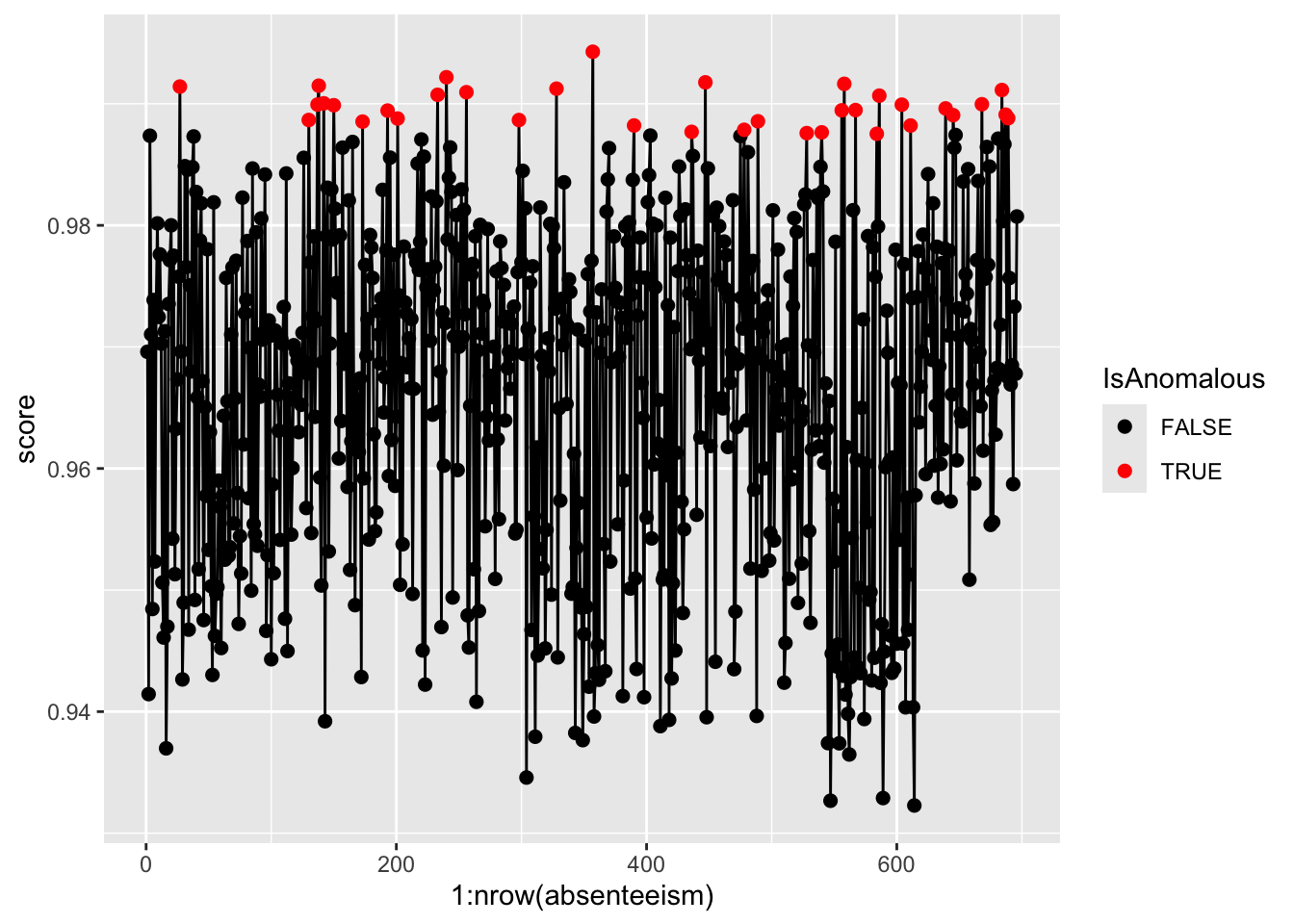
Step 5. Further Analysis with Plots
Analyze the distribution of anomalies using box and bar plots to explore differences in numeric and categorical data between normal and anomalous observations.
absenteeism.rf <- select(absenteeism.rf, -score)
anomaly.boxplot(data = absenteeism.rf, anomaly_indicator = "IsAnomalous")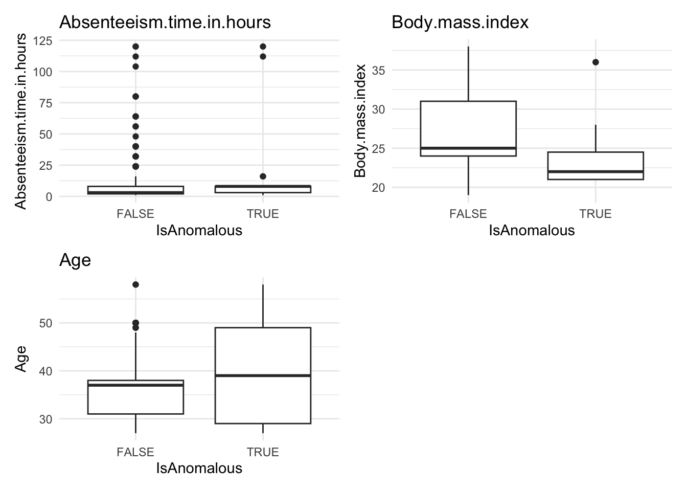
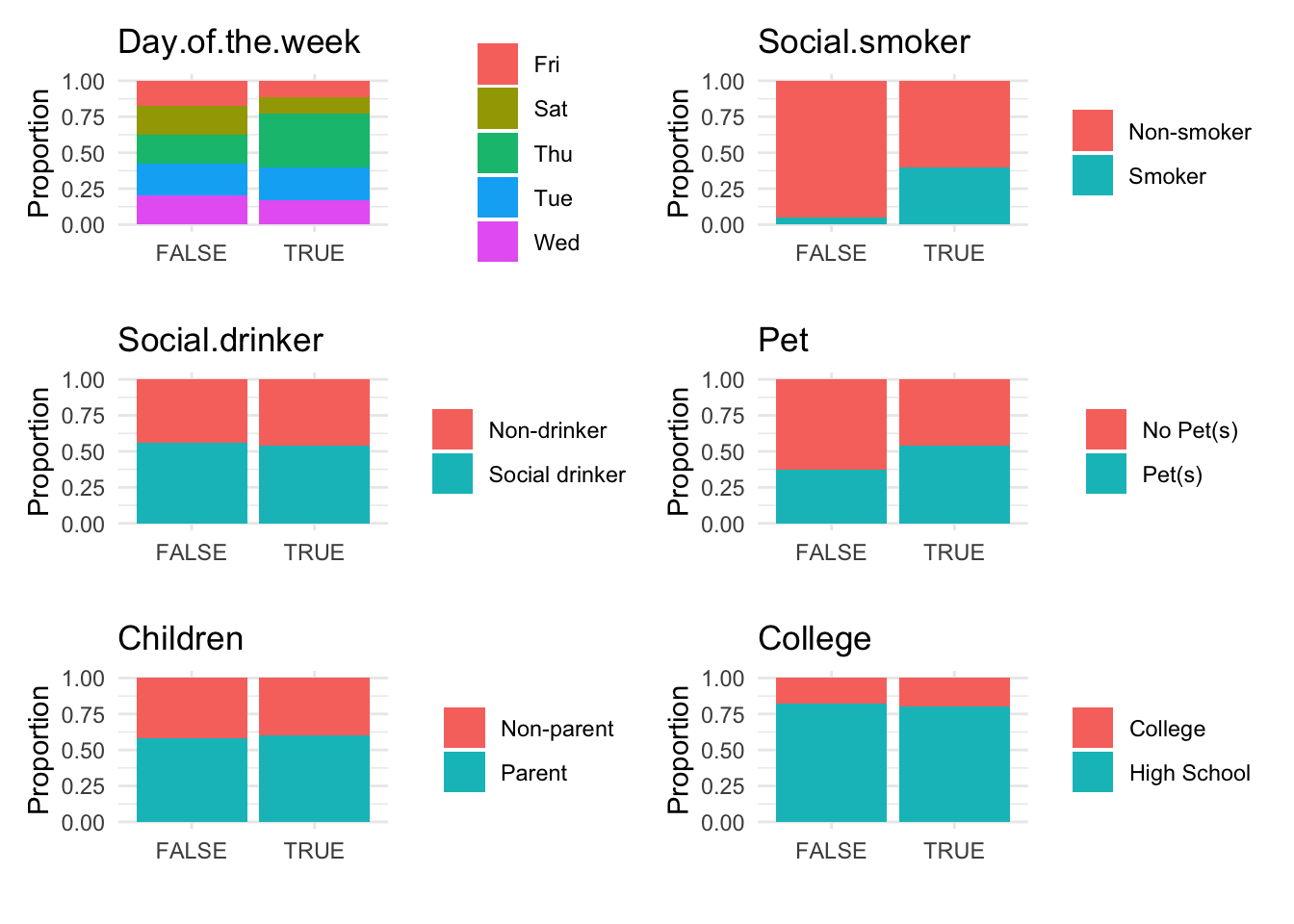
Anomalous observations typically exhibit a lower average BMI, and they have a higher proportion of smokers and pet owners. Other metrics are similar for both anomalous and non-anomalous groups.