10.2 Modeling Absenteeism
10.2.1 Linear Model Prediction of Absenteeism Time in Hours
10.2.1.1 Model with all predictors
To predict Absenteeism.time.in.hours and understand its underlying factors, we use a linear regression model. The model identifies key variables that influence absenteeism by assessing their statistical significance and effect sizes.
# Initial linear model excluding some predictors
Absenteeism.lm <- lm(Absenteeism.time.in.hours ~ .
                     - Number.of.absence
                     - High.absenteeism,
                     data = Absenteeism.by.employee)
summ(Absenteeism.lm)| Observations | 33 |
| Dependent variable | Absenteeism.time.in.hours |
| Type | OLS linear regression |
| F(6,26) | 1.54 |
| R² | 0.26 |
| Adj. R² | 0.09 |
| Est. | S.E. | t val. | p | |
|---|---|---|---|---|
| (Intercept) | 36.69 | 14.18 | 2.59 | 0.02 |
| Body.mass.index | -0.44 | 0.52 | -0.84 | 0.41 |
| Age | -0.37 | 0.30 | -1.22 | 0.23 |
| Social.smokerSmoker | -12.21 | 5.36 | -2.28 | 0.03 |
| Social.drinkerSocial drinker | 1.05 | 4.78 | 0.22 | 0.83 |
| PetPet(s) | -4.12 | 5.49 | -0.75 | 0.46 |
| ChildrenParent | 7.11 | 5.74 | 1.24 | 0.23 |
| Standard errors: OLS |
Breaking Down the Code
- The
lm()function fits a linear regression model, predictingAbsenteeism.time.in.hoursusing all available variables inAbsenteeism.by.employeeexceptNumber.of.absenceandHigh.absenteeism. summ()from the jtools package provides an enhanced summary of the linear model, showing estimates, standard errors, t-values, and p-values, making interpretation straightforward.
Results Explanation:
- Model Info: The analysis includes 33 observations.
- Model Fit: The overall fit of the model is weak (F(6,26) = 1.54, p = 0.21, R² = 0.26, Adj. R² = 0.09), indicating that the variables explain only 26% of the variability in absenteeism hours. Adjustments for the number of predictors lead to a lower adjusted R² of 0.09.
- Coefficients: The intercept and
Social.smokerSmokerare statistically significant (p < 0.05), suggesting a baseline absenteeism time when all predictors are zero and a notable decrease in absenteeism for smokers, respectively.
10.2.1.2 Refine the model variable selection
Next, we refine the model using stepwise regression based on the AIC criterion to select the most informative variables. Stepwise regression iteratively adds or removes predictors based on their statistical significance to optimize the AIC value. Lower AIC values generally indicate a better model fit given the number of parameters.
## Start:  AIC=168.35
## Absenteeism.time.in.hours ~ (Number.of.absence + Body.mass.index +
##     Age + Social.smoker + Social.drinker + Pet + Children + High.absenteeism) -
##     Number.of.absence - High.absenteeism
##
##                   Df Sum of Sq    RSS    AIC
## - Social.drinker   1      6.56 3553.7 166.41
## - Pet              1     76.61 3623.8 167.06
## - Body.mass.index  1     97.36 3644.5 167.25
## - Age              1    201.96 3749.1 168.18
## - Children         1    209.17 3756.3 168.25
## <none>                         3547.2 168.35
## - Social.smoker    1    706.50 4253.7 172.35
##
## Step:  AIC=166.42
## Absenteeism.time.in.hours ~ Body.mass.index + Age + Social.smoker +
##     Pet + Children
##
##                   Df Sum of Sq    RSS    AIC
## - Body.mass.index  1     91.08 3644.8 165.25
## - Pet              1    117.44 3671.2 165.49
## <none>                         3553.7 166.41
## - Age              1    225.80 3779.5 166.45
## - Children         1    281.88 3835.6 166.93
## - Social.smoker    1    702.21 4256.0 170.37
##
## Step:  AIC=165.25
## Absenteeism.time.in.hours ~ Age + Social.smoker + Pet + Children
##
##                 Df Sum of Sq    RSS    AIC
## - Pet            1    158.56 3803.4 164.66
## <none>                       3644.8 165.25
## - Children       1    256.68 3901.5 165.50
## - Age            1    348.79 3993.6 166.27
## - Social.smoker  1    617.23 4262.0 168.41
##
## Step:  AIC=164.66
## Absenteeism.time.in.hours ~ Age + Social.smoker + Children
##
##                 Df Sum of Sq    RSS    AIC
## - Children       1    126.79 3930.2 163.74
## <none>                       3803.4 164.66
## - Age            1    455.58 4259.0 166.39
## - Social.smoker  1    532.00 4335.4 166.98
##
## Step:  AIC=163.74
## Absenteeism.time.in.hours ~ Age + Social.smoker
##
##                 Df Sum of Sq    RSS    AIC
## <none>                       3930.2 163.74
## - Age            1    362.84 4293.0 164.65
## - Social.smoker  1    451.76 4381.9 165.33
Stepwise regression results Explanation:
- The model simplifies by sequentially removing predictors that do not significantly improve the model, such as
Social.drinkerandPet. - The final model focuses on
AgeandSocial.smoker, indicating these are the most significant predictors under the AIC criterion.
Refined Model Output:
| Observations | 33 |
| Dependent variable | Absenteeism.time.in.hours |
| Type | OLS linear regression |
| F(2,30) | 3.35 |
| R² | 0.18 |
| Adj. R² | 0.13 |
| Est. | S.E. | t val. | p | |
|---|---|---|---|---|
| (Intercept) | 30.59 | 10.46 | 2.92 | 0.01 |
| Age | -0.44 | 0.26 | -1.66 | 0.11 |
| Social.smokerSmoker | -9.07 | 4.89 | -1.86 | 0.07 |
| Standard errors: OLS |
- Model Info: The final model also consists of 33 observations.
- Model Fit: This refined model has a slightly improved fit (F(2,30) = 3.35, p = 0.05), with an R² of 0.18 and an adjusted R² of 0.13, indicating modest explanatory power.
- Coefficients: Both
AgeandSocial.smokerSmokerare the remaining predictors, withAgeshowing a negative association with absenteeism time (more absenteeism with increasing age) and smoking status reducing absenteeism, both marginally significant.
10.2.1.3 Brief Model Diagnotics
Finally, we assess the quality of the model by examining the residuals versus fitted values.
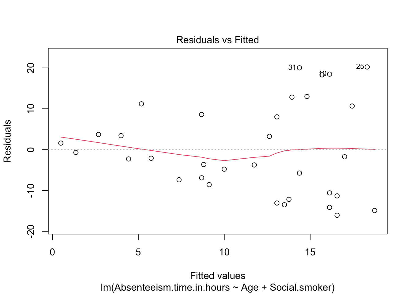
Breaking Down the Code This plot visualizes the residuals (differences between observed and predicted values) against the fitted values (predicted values). It is used to check for patterns that could suggest issues like heteroscedasticity.
Analysis of Results: - The plot indicates potential heteroscedasticity, where the variance of residuals varies with the level of the fitted values. This condition can invalidate the assumptions of constant variance in standard linear regression models. - Combined with the modest R² values, these issues suggest that linear regression might not be the most reliable method for analyzing this data, possibly requiring alternative methods or transformations to better capture the underlying patterns.
10.2.2 Logistic Model Prediction of Absenteeism
We employ logistic regression to model the probability that employees fall into categories of “High Absenteeism” or “Low Absenteeism” based on various predictors. Logistic regression is useful for binary outcomes and provides probabilities as outputs, which can be thresholded at a particular value (commonly 0.5) to classify observations.
10.2.2.1 Model with All Predictors
We employ a logistic regression model, using the glm() function with a binomial family, to predict High.absenteeism. In this model, we exclude the variables Absenteeism.time.in.hours and Number.of.absence from the predictors. These exclusions are made because these variables are derived from the dependent variable, which could lead to multicollinearity or redundancy, potentially skewing the model’s accuracy and interpretability.
Absenteeism.Logit <- glm(High.absenteeism ~ .
            - Absenteeism.time.in.hours
            - Number.of.absence,
            data = Absenteeism.by.employee,
            family = "binomial")
Breaking Down the Code
The R code you provided fits a logistic regression model to predict a binary outcome, labeled High.absenteeism, which categorizes employees based on their absenteeism rates. Here’s a breakdown of each component of the code:
Absenteeism.Logit <- glm(High.absenteeism ~ .
            - Absenteeism.time.in.hours
            - Number.of.absence,
            data = Absenteeism.by.employee,
family = "binomial")glm(): This function is used to fit generalized linear models, a class of models that includes logistic regression. The type of model is specified by thefamilyparameter.High.absenteeism ~ .: This part of the formula specifies thatHigh.absenteeismis the dependent variable we are trying to predict. The~ .indicates that all other variables in the dataset should be considered as predictors.- Absenteeism.time.in.hours - Number.of.absence: These terms are preceded by a minus sign, which means they are explicitly excluded from the set of predictor variables.data = Absenteeism.by.employee: Specifies the dataset from which variables are taken. In this case, it’sAbsenteeism.by.employee, which presumably contains the employee attendance data.family = "binomial": Indicates that the model should be fit using the binomial family, which is used for binary outcomes. In logistic regression, this setting specifies that the link function (the function that relates the linear predictor to the mean of the distribution function) is the logit function, suitable for binary data.
This model is structured to examine the influence of various predictors on the likelihood of an employee having high absenteeism, while ensuring that the analysis does not include redundant or inappropriate predictors.
| Observations | 33 |
| Dependent variable | High.absenteeism |
| Type | Generalized linear model |
| Family | binomial |
| Link | logit |
| 𝛘²(6) | 9.79 |
| p | 0.13 |
| Pseudo-R² (Cragg-Uhler) | 0.34 |
| Pseudo-R² (McFadden) | 0.21 |
| AIC | 49.92 |
| BIC | 60.40 |
| Est. | S.E. | z val. | p | |
|---|---|---|---|---|
| (Intercept) | -3.79 | 3.28 | -1.15 | 0.25 |
| Body.mass.index | 0.13 | 0.11 | 1.13 | 0.26 |
| Age | 0.03 | 0.06 | 0.50 | 0.61 |
| Social.smokerSmoker | 2.77 | 1.41 | 1.97 | 0.05 |
| Social.drinkerSocial drinker | -0.34 | 0.93 | -0.36 | 0.72 |
| PetPet(s) | 1.80 | 1.31 | 1.37 | 0.17 |
| ChildrenParent | -3.11 | 1.55 | -2.00 | 0.05 |
| Standard errors: MLE |
Model Information: - Observations: 33 - Dependent Variable: High.absenteeism - Type: Generalized linear model with a logit link function (logistic regression).
Model Fit: - χ²(6) = 9.79, p = 0.13: The chi-square test indicates that the model as a whole is not statistically significant at conventional levels. - Pseudo-R² (Cragg-Uhler) = 0.34 and Pseudo-R² (McFadden) = 0.21: These values suggest a moderate fit, showing that the model explains some, but not all, of the variability in absenteeism classification. - AIC = 49.92, BIC = 60.40: These information criteria suggest the model’s relative quality of fit to the data; lower values are better.
Coefficients Analysis:
- Most variables are not statistically significant, indicating a weak association with the likelihood of high absenteeism. Notable exceptions include Social.smokerSmoker and ChildrenParent, both at the boundary of significance, suggesting potential areas for further investigation.
10.2.2.2 Refine the Model: Variable Selection
we utilize Stepwise regression to automated process of adding and removing predictors based on their statistical significance.
## Start:  AIC=49.92
## High.absenteeism ~ (Number.of.absence + Absenteeism.time.in.hours +
##     Body.mass.index + Age + Social.smoker + Social.drinker +
##     Pet + Children) - Absenteeism.time.in.hours - Number.of.absence
##
##                   Df Deviance    AIC
## - Social.drinker   1   36.054 48.054
## - Age              1   36.179 48.179
## - Body.mass.index  1   37.265 49.265
## <none>                 35.924 49.924
## - Pet              1   38.179 50.179
## - Social.smoker    1   41.436 53.436
## - Children         1   41.574 53.574
##
## Step:  AIC=48.05
## High.absenteeism ~ Body.mass.index + Age + Social.smoker + Pet +
##     Children
##
##                   Df Deviance    AIC
## - Age              1   36.363 46.363
## - Body.mass.index  1   37.272 47.272
## <none>                 36.054 48.054
## - Pet              1   38.958 48.958
## - Social.smoker    1   41.457 51.457
## - Children         1   42.951 52.951
##
## Step:  AIC=46.36
## High.absenteeism ~ Body.mass.index + Social.smoker + Pet + Children
##
##                   Df Deviance    AIC
## - Body.mass.index  1   37.764 45.764
## <none>                 36.363 46.363
## - Pet              1   39.297 47.297
## - Social.smoker    1   41.938 49.938
## - Children         1   42.974 50.974
##
## Step:  AIC=45.76
## High.absenteeism ~ Social.smoker + Pet + Children
##
##                 Df Deviance    AIC
## <none>               37.764 45.764
## - Pet            1   41.233 47.233
## - Social.smoker  1   42.229 48.229
## - Children       1   43.485 49.485
Stepwise Regression Results:
The results detail a stepwise regression process aimed at optimizing a logistic regression model by minimizing the Akaike Information Criterion (AIC). Initially, the model includes several predictors, starting with an AIC of 49.92. Through the stepwise removal of predictors that contribute the least to the model’s explanatory power, the AIC is progressively lowered. Significant reductions are achieved by first removing Social.drinker, which lowers the AIC to 48.054, and then by excluding Age, which further reduces the AIC to 46.363. The final variable selection includes Social smoker, Pet, and Children, as removing any of these results in a higher AIC, indicating their importance in the model. The process concludes with a refined model that effectively balances simplicity and explanatory power, with a final AIC of 45.76. This model retains only the most statistically significant predictors, providing a streamlined yet informative analysis of factors influencing high absenteeism.
Refined Model Output:
| Observations | 33 |
| Dependent variable | High.absenteeism |
| Type | Generalized linear model |
| Family | binomial |
| Link | logit |
| 𝛘²(3) | 7.95 |
| p | 0.05 |
| Pseudo-R² (Cragg-Uhler) | 0.29 |
| Pseudo-R² (McFadden) | 0.17 |
| AIC | 45.76 |
| BIC | 51.75 |
| Est. | S.E. | z val. | p | |
|---|---|---|---|---|
| (Intercept) | 0.30 | 0.66 | 0.45 | 0.65 |
| Social.smokerSmoker | 2.28 | 1.24 | 1.83 | 0.07 |
| PetPet(s) | 1.95 | 1.21 | 1.62 | 0.11 |
| ChildrenParent | -2.63 | 1.30 | -2.03 | 0.04 |
| Standard errors: MLE |
Model Fit and Statistical Significance: The model’s goodness-of-fit, as indicated by a chi-square value of 7.95 with a p-value of 0.05, suggests that the model as a whole is statistically significant at the conventional 0.05 level. This indicates that the model provides a better fit to the data than a model with no predictors.
Coefficient Analysis: - Intercept: The estimate is 0.30 with a standard error of 0.66, resulting in a z-value of 0.45 and a p-value of 0.65. This indicates that the baseline log odds of high absenteeism (when all predictors are zero) is not significantly different from zero. - Social Smoker: The coefficient of 2.28 with a standard error of 1.24 and a z-value of 1.83 suggests that being a smoker increases the log odds of being classified as a high absentee, although this result is marginally significant (p = 0.07). - Pet(s): With a coefficient of 1.95, a standard error of 1.21, and a z-value of 1.62, this predictor also shows a tendency towards increasing the likelihood of high absenteeism, but the result is not statistically significant (p = 0.11). - Children (Parent): This variable has a coefficient of -2.63, indicating that parents are less likely to be classified under high absenteeism, with a standard error of 1.30 and a z-value of -2.03, making it statistically significant (p = 0.04).
Pseudo-R² Values: - The Cragg-Uhler Pseudo-R² is 0.29 and McFadden’s Pseudo-R² is 0.17, both of which are modest. These values indicate that while the model explains some variability in high absenteeism, a significant portion remains unexplained, suggesting that absenteeism is influenced by other unmeasured factors or that the relationship is not purely logistic.
Overall, the model suggests that certain lifestyle factors like smoking and having children are important in predicting high absenteeism, though the moderate Pseudo-R² values and the marginal significance of some predictors call for cautious interpretation of the results.