11.3 Data Mining Techniques
Five core techniques form the foundation of data mining practice (Larose and Larose 2014). Each addresses a different type of question.
11.3.1 Classification
Classification assigns observations to predefined categories. Given a set of labeled training data, a classification model learns to predict the category of new observations.
Common algorithms: Decision trees, support vector machines (SVM), naive Bayes, k-nearest neighbors (KNN), and neural networks.
Business application: In banking, classification models assess credit risk by analyzing income, employment history, and repayment records to categorize loan applicants as “high risk” or “low risk.” This informs lending decisions, interest rates, and required collateral.
11.3.2 Clustering
Clustering groups similar observations together without predefined labels — it discovers natural groupings in the data rather than predicting known categories.
Common algorithms: K-means, hierarchical clustering, DBSCAN, and spectral clustering.
Business application: Retailers use clustering to segment customers by purchasing behavior. One cluster might represent frequent, high-spending shoppers; another might represent occasional bargain hunters. Each segment receives tailored marketing, improving engagement and conversion rates.
11.3.3 Association Rule Learning
Association rule learning discovers relationships between variables in transactional data — which items tend to appear together.
Common algorithms: Apriori, FP-Growth, and Eclat.
Business application: Market basket analysis reveals that customers who buy pasta frequently also buy tomato sauce and cheese. Retailers use these rules to optimize store layouts, create bundle promotions, and power online recommendation engines.
11.3.4 Regression in Data Mining
While regression was introduced in Chapter 9 as a statistical modeling technique, it also plays a role in data mining when applied to large-scale prediction tasks with many potential predictors.
Common techniques: Linear regression, polynomial regression, ridge and lasso regression (for regularization), and support vector regression.
Business application: A clothing retailer uses regression to forecast seasonal sales by incorporating past sales figures, weather data, economic indicators, and promotional calendars. Accurate forecasts drive inventory decisions, staffing plans, and marketing budgets.
11.3.5 Anomaly Detection
Anomaly detection identifies observations that deviate significantly from the expected pattern — the data points that do not fit.
Common algorithms: Statistical methods (z-scores), isolation forests, one-class SVM, DBSCAN (points not in any cluster), and autoencoders (neural networks that flag high reconstruction error).
Business application: Financial institutions use anomaly detection to flag potentially fraudulent transactions — a sudden large international purchase on an account that typically makes small local transactions. In network security, anomaly detection identifies unusual traffic patterns that may indicate a cyberattack.
A simple R demonstration of anomaly detection using z-scores:
# Detect anomalies in mtcars MPG using z-scores
mpg_mean <- mean(mtcars$mpg)
mpg_sd <- sd(mtcars$mpg)
mtcars$z_score <- (mtcars$mpg - mpg_mean) / mpg_sd
mtcars$anomaly <- abs(mtcars$z_score) > 2

# Show the flagged anomalies
mtcars |>
  filter(anomaly) |>
  select(mpg, wt, cyl, z_score) |>
arrange(desc(abs(z_score)))| mpg | wt | cyl | z_score |
|---|---|---|---|
| 33.9 | 1.83 | 4 | 2.29 |
| 32.4 | 2.2 | 4 | 2.04 |
Observations with z-scores beyond ±2 are flagged as potential anomalies — they fall in the tails of the distribution. In Chapter 12, we apply more sophisticated anomaly detection methods (linear regression residuals, KNN, and random forests) to the Absenteeism dataset.
A brief demonstration of k-means clustering:
# Cluster cars by fuel efficiency and weight
car_data <- mtcars |> select(mpg, wt) |> scale()
set.seed(42)
km <- kmeans(car_data, centers = 3, nstart = 25)

mtcars |>
  mutate(Cluster = factor(km$cluster)) |>
  ggplot(aes(x = wt, y = mpg, color = Cluster)) +
  geom_point(size = 3) +
  labs(title = "K-Means Clustering: Cars by Weight and MPG",
       x = "Weight (1000 lbs)", y = "Miles per Gallon") +
  theme_minimal()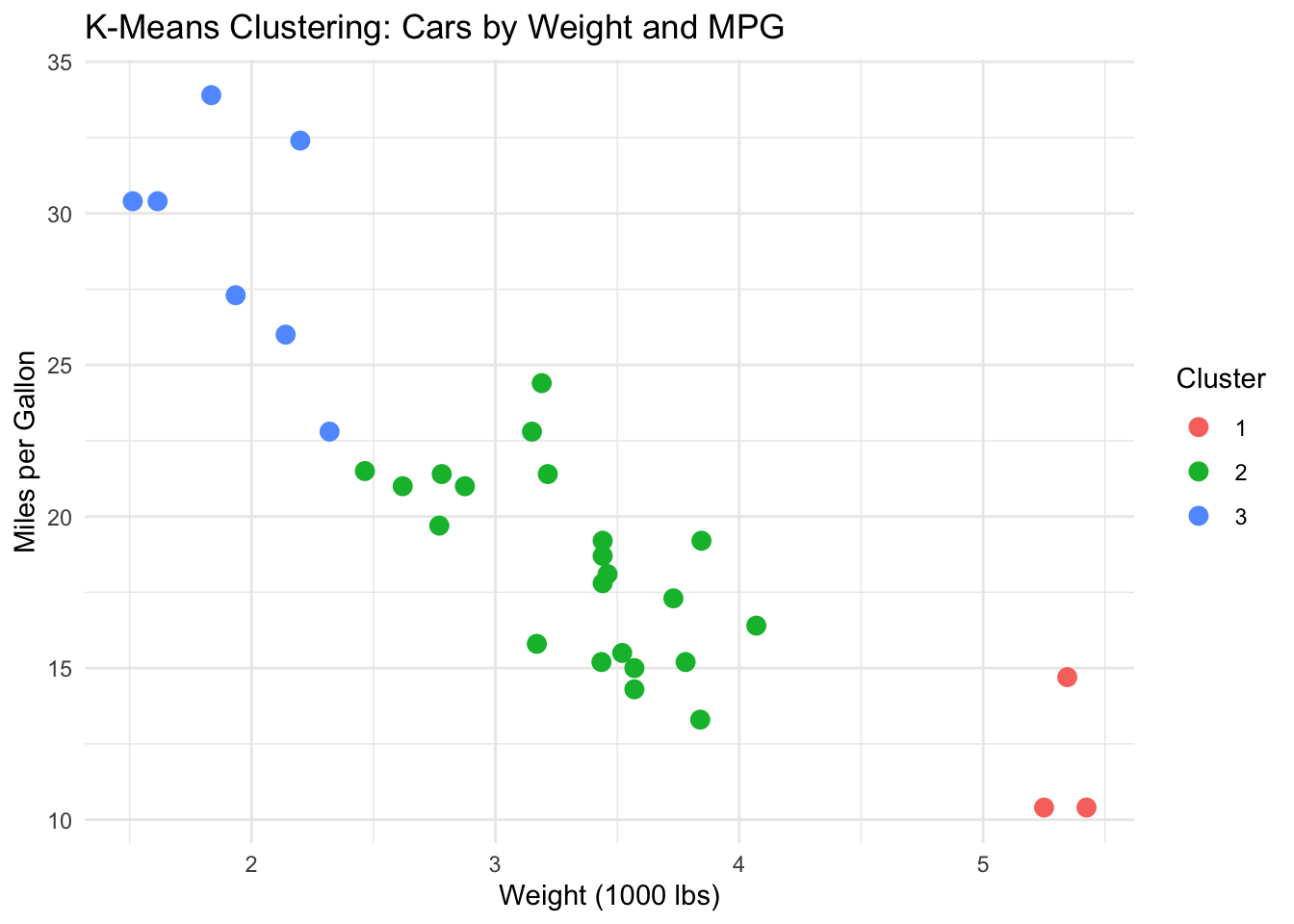
The algorithm discovers three natural groups without being told what they are — lightweight fuel-efficient cars, mid-range cars, and heavy gas-guzzlers. A BI analyst might apply the same technique to segment employees by absence patterns, customers by purchasing behavior, or products by sales characteristics.