3 Data, Datasets, and Data Structure

PRELIMINARY AND INCOMPLETE

Understanding data is fundamental to effective analysis. In the realm of business analytics, data comes in various forms, each with its own set of characteristics and applications. This chapter will guide you through the different types of data, the structures in which data can be organized, and how these concepts translate into practical use within R.

3.1 Chapter Goals

Upon concluding this chapter, readers will be equipped with the skills to:

Identify and recall the different types of data and data structures in R.
Explain the significance of various data types and structures in the context of business analytics.
Import, clean, and transform common business datasets using R.
Distinguish between different data structures and select the appropriate one for specific analytical tasks.
Assess the quality and suitability of datasets for analysis after performing data cleaning and transformation.
Construct and export well-structured datasets that are ready for advanced analysis and reporting.

3.2 Types of Data

Understanding the types of data is fundamental to performing effective analysis. Data can be broadly categorized based on its characteristics, with each type requiring different analytical approaches. The primary types of data are quantitative and qualitative, each of which plays a unique role in statistical analysis.

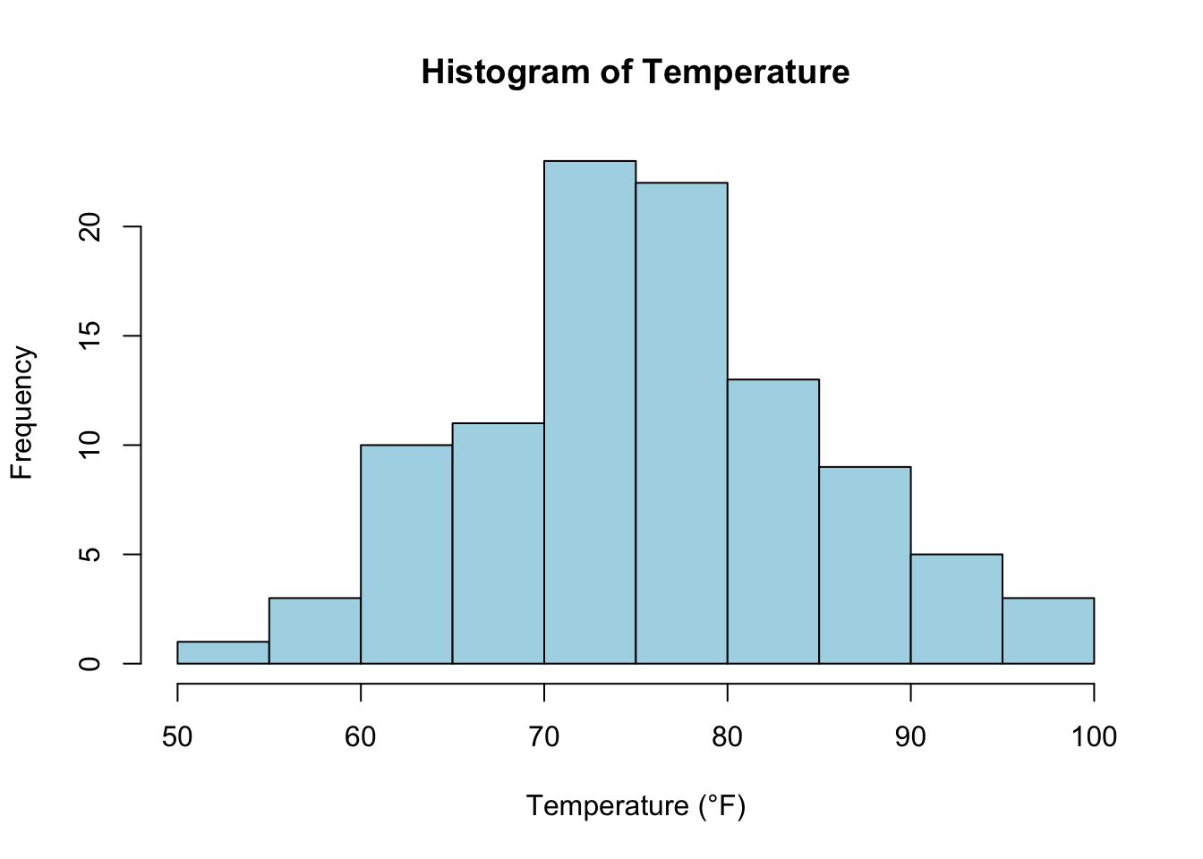
Quantitative data represents numerical values that can be measured and is further subdivided into continuous and discrete data. Continuous data includes values that can take any real number within a given range. These values often arise from measurements and can include decimals or fractions. For instance, the temperature of a city measured over time, the revenue generated by a company, or the height of individuals are examples of continuous data. In R, you can visualize continuous data using histograms or density plots. For example, consider the following code that generates a histogram of a continuous variable, such as temperature:

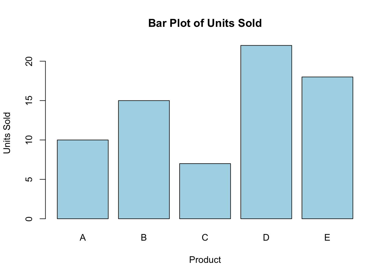
On the other hand, discrete data consists of values that represent counts and can only take specific numbers, usually whole numbers. These values typically result from counting occurrences of specific events or entities. For example, the number of employees in a department, the units sold by a retailer, or the number of customer complaints received in a month are all discrete data. Discrete data can be effectively visualized using bar charts. Here’s an example in R that visualizes the number of units sold:

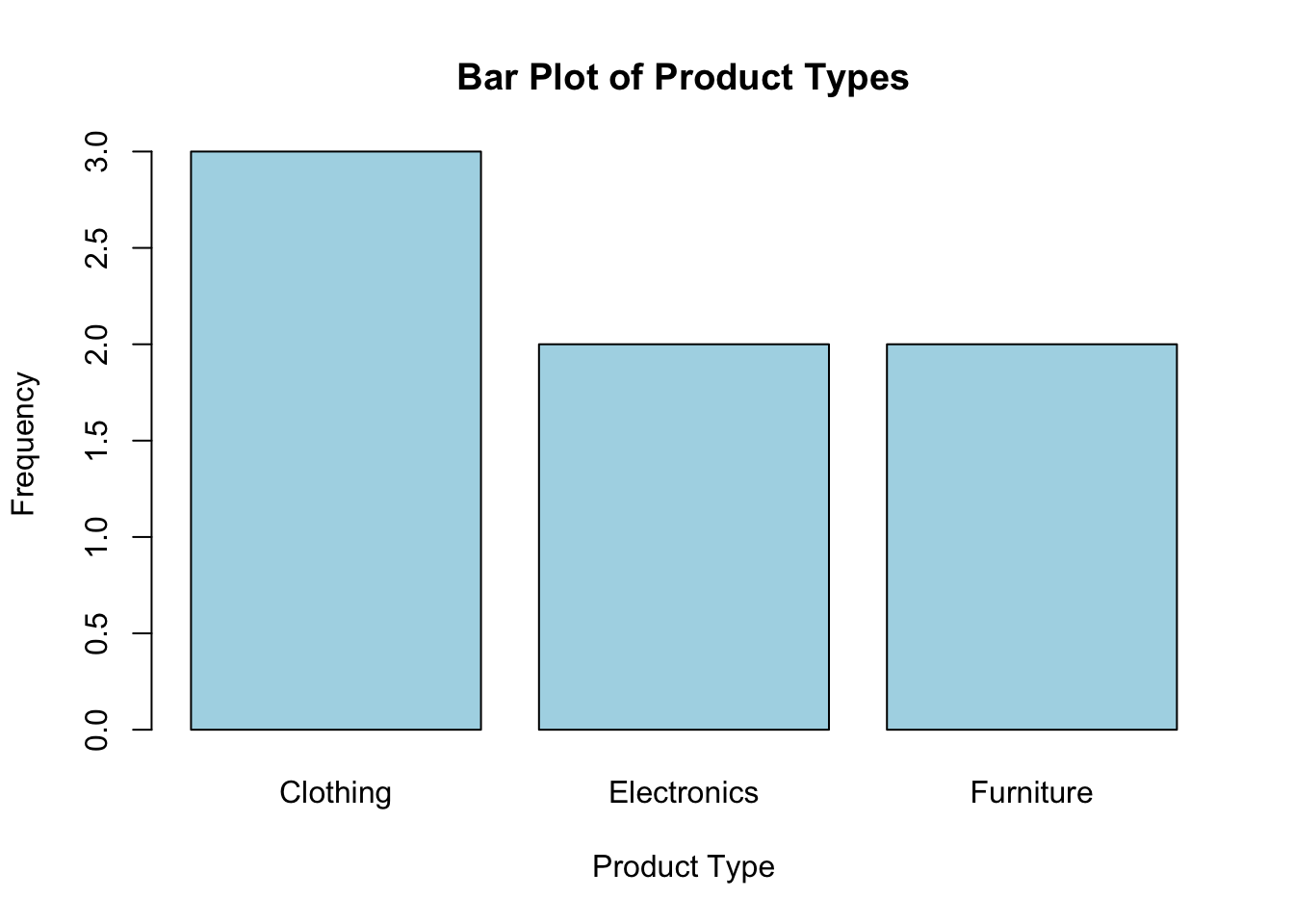
Qualitative data, also known as categorical data, represents attributes or categories rather than numerical values. This type of data is subdivided into nominal and ordinal data. Nominal data consists of categories that do not have any inherent order or ranking. For example, product types such as electronics, furniture, and clothing, or colors like red, blue, and green, are nominal data. The frequency of each category can be visualized using pie charts or bar charts. Consider the following R code that creates a bar chart for product types:

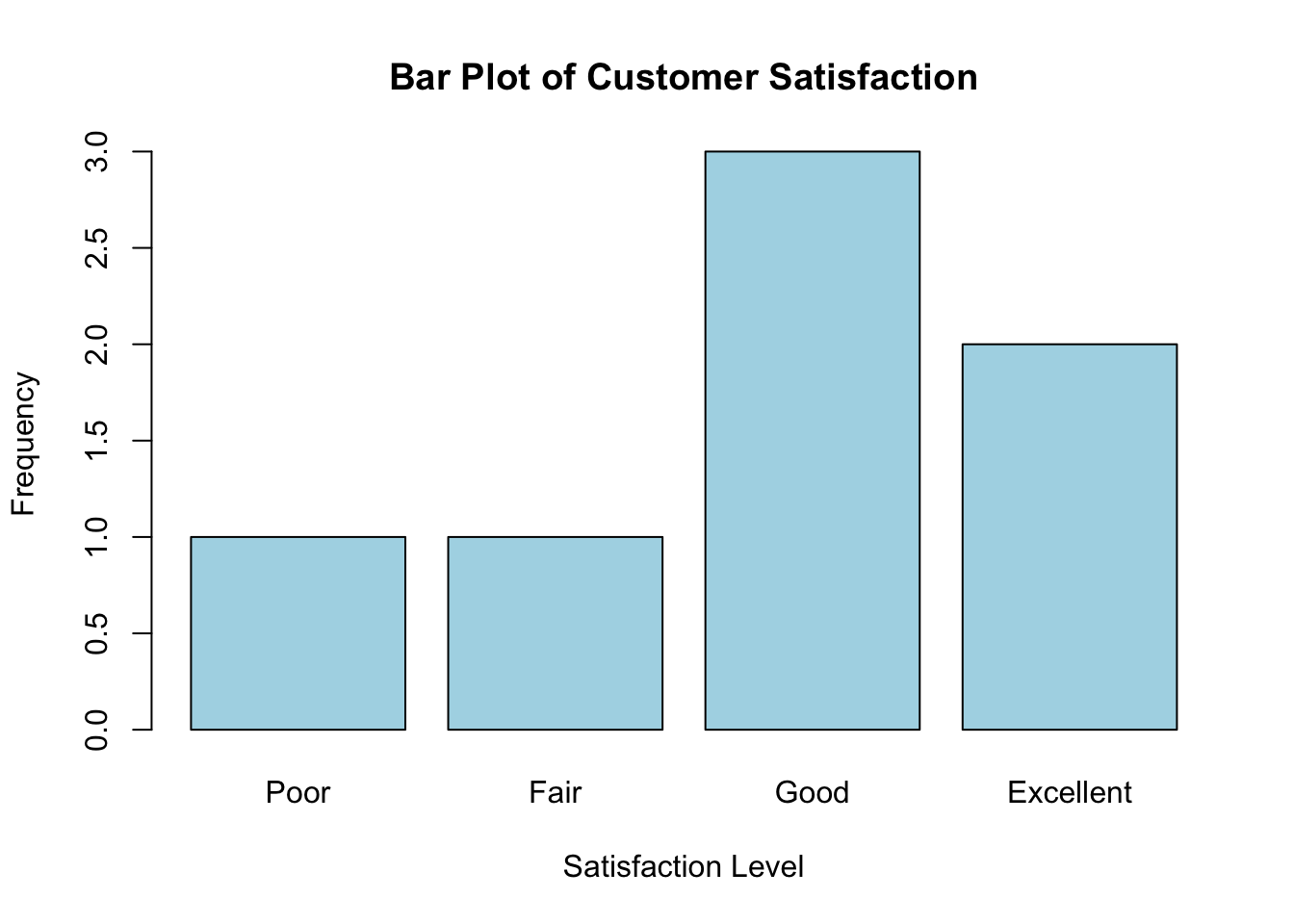
Ordinal data, on the other hand, represents categories with a meaningful order, though the intervals between the categories are not defined or consistent. For instance, customer satisfaction ratings such as poor, fair, good, and excellent, or education levels like high school, bachelor’s degree, and master’s degree, are ordinal data because they imply a rank or order. However, the difference between these categories is not measurable or uniform. Ordinal data can be visualized using ordered bar charts. The following R code demonstrates how to create an ordered bar chart for customer satisfaction ratings:

Understanding the distinctions between these types of data is crucial for selecting appropriate statistical methods and ensuring accurate interpretations of results. Quantitative and qualitative data offer unique insights and pose specific challenges, making it essential to recognize the nature of your data before proceeding with any analysis. Whether you’re dealing with continuous temperature readings, discrete counts of product units sold, or ordinal satisfaction ratings, the right analytical approach will depend on correctly identifying the type of data at hand.

3.3 Data Structures in R

R offers a variety of data structures to organize and manage different types of data. Each structure serves specific analytical purposes and allows for various operations. Below are the main data structures in R, along with examples, explanations of the syntax, and methods to access data within each structure.

3.3.1 Vectors

A vector is a one-dimensional array that holds data of a single type. Vectors are the simplest R structure and can contain numeric, character, or logical data.

Example: Creating and Accessing a Numeric Vector
To create a vector, you can use the c() function, which combines values into a vector. For example, the following R code creates a numeric vector named sales_vector, which contains sales figures:

# Creating a numeric vector
sales_vector <- c(120, 150, 90, 100, 130, 170, 200)
sales_vector

[1] 120 150  90 100 130 170 200

To access an element within a vector, use square brackets [] with the index of the element. For example, sales_vector[1] accesses the first element of the vector. In R, indexing starts at 1, so sales_vector[1] returns 120:

sales_vector[1]

[1] 120

3.3.2 Matrices

Matrices extend vectors to two dimensions, where each element is of the same type. They are useful for mathematical operations across rows and columns.

Example: Creating and Accessing a Numeric Matrix
The matrix() function creates a matrix. The first argument is the vector of elements, while nrow specifies the number of rows, ncol specifies the number of columns, and byrow = TRUE indicates that the matrix should be filled by rows:

# Creating a numeric matrix
sales_matrix <- matrix(c(120, 150, 90, 100, 130, 170, 200, 210, 180), 
                       nrow = 3, 
                       ncol = 3, 
                       byrow = TRUE)

To access an element within a matrix, use square brackets with the row and column indices, separated by a comma. For example, sales_matrix[1, 2] accesses the element in the first row and second column, returning 150:

element <- sales_matrix[1, 2]

3.3.3 Data Frames

Data frames are two-dimensional structures where each column can contain different types of data. They are the most common structure for storing datasets in R.

Example: Creating and Accessing a Data Frame
The data.frame() function creates a data frame. Each argument represents a column in the data frame. For example, the following R code creates a data frame named sales_data, where Product is a character vector, and Sales_Q1 and Sales_Q2 are numeric vectors:

# Creating a data frame
sales_data <- data.frame(
  Product = c("A", "B", "C", "D", "E"),
  Sales_Q1 = c(120, 150, 90, 100, 130),
  Sales_Q2 = c(170, 200, 140, 180, 190)
)

To access an entire column, you can use the $ operator followed by the column name. For example, sales_data$Sales_Q1 accesses the Sales_Q1 column:

sales_q1 <- sales_data$Sales_Q1
sales_q1

[1] 120 150  90 100 130

To access a specific element, use square brackets with the row index and column name. For example, sales_data[2, "Sales_Q1"] returns 150:

# Accessing a specific element by row and column
specific_sale <- sales_data[2, "Sales_Q1"]
specific_sale

[1] 150

3.3.4 Lists

A list can contain elements of different types, including vectors, matrices, data frames, and even other lists. This makes lists highly flexible for storing complex data structures.

Example: Creating and Accessing a List
The list() function creates a list by combining different elements, such as vectors, matrices, and data frames. For example, the following R code creates a list named sales_list, combining product_vector, sales_vector, and sales_data (Note that for this code to run you will need these objects to exist):

# Creating the list
sales_list <- list(
  Products = product_vector,
  Sales = sales_vector,
  Data = sales_data
)

# Viewing the structure of the list
str(sales_list)

List of 3
 $ Products: chr [1:5] "Canon EOS R5" "Nikon Z7 II" "Sony Alpha A7R IV" "Fujifilm X-T4" ...
 $ Sales   : num [1:5] 215 415 264 453 476
 $ Data    :'data.frame':   20 obs. of  3 variables:
  ..$ Product: chr [1:20] "Canon EOS R5" "Canon EOS R5" "Canon EOS R5" "Canon EOS R5" ...
  ..$ Region : chr [1:20] "North" "South" "East" "West" ...
  ..$ Sales  : num [1:20] 55 103 139 105 96 146 95 118 107 60 ...

To access elements within a list, you can use the $ operator followed by the element name. For example, sales_list$Sales accesses the Sales element:

sales_list$Sales

[1] 215 415 264 453 476

Alternatively, you can use double square brackets [[ ]] with the position of the element (e.g., sales_list[[1]]), which returns the first element of the list:

sales_list[[1]]

[1] "Canon EOS R5"        "Nikon Z7 II"         "Sony Alpha A7R IV"  
[4] "Fujifilm X-T4"       "Panasonic Lumix GH5"

In R, lists are a flexible data structure that can store different types of elements, including other lists. Accessing elements within a list can be done using either single square brackets [] or double square brackets [[ ]], but they behave differently:

Single Square Brackets []: When you use single square brackets with a list, R returns a sublist containing the specified elements. This means that the result is still a list, even if it only contains one element. For example, sales_list[1] would return a list containing the first element of sales_list, but the result itself is a list:

sales_list[1]

$Products
[1] "Canon EOS R5"        "Nikon Z7 II"         "Sony Alpha A7R IV"  
[4] "Fujifilm X-T4"       "Panasonic Lumix GH5"

Double Square Brackets [[ ]]: When you use double square brackets with a list, R directly extracts the specified element itself, rather than returning it as a sublist. This is useful when you want to work with the actual element within the list, such as a vector or data frame, rather than with a list that contains that element. For example, sales_list[[1]] would return the actual vector stored as the first element of sales_list:

sales_list[[1]]

[1] "Canon EOS R5"        "Nikon Z7 II"         "Sony Alpha A7R IV"  
[4] "Fujifilm X-T4"       "Panasonic Lumix GH5"

In summary, use [] when you want to retrieve a sublist (i.e., a list of elements), and use [[ ]] when you want to directly access and manipulate the actual content of the list element.

3.3.5 Factors

Factors are used for storing categorical data and are especially useful for handling ordinal data. They ensure proper treatment of categorical variables in statistical models.

Example: Creating and Accessing a Factor
The factor() function creates a factor, a special type of vector used for categorical data. For example, the following R code creates a factor named satisfaction_levels:

# Creating a factor
satisfaction_levels <- factor(c("High", "Medium", "Low", "Medium", "High"))

# Accessing levels of the factor
levels_satisfaction <- levels(satisfaction_levels)

# Accessing a specific level by position
first_level <- satisfaction_levels[1]

# Printing the accessed levels and specific level
print(levels_satisfaction)

[1] "High"   "Low"    "Medium"

print(first_level)

[1] High
Levels: High Low Medium

To access a specific level within a factor, use square brackets with the index of the level (e.g., satisfaction_levels[1]), which returns High.

Example: Creating and Accessing an Ordered Factor
To create an ordered factor, use the factor() function with levels and ordered arguments. For example:

# Creating an ordered factor
ordered_levels <- factor(c("Low", "Medium", "High", "Medium", "Low"),
                         levels = c("Low", "Medium", "High"),
                         ordered = TRUE)

# Checking if the factor is ordered
is_ordered <- is.ordered(ordered_levels)

# Accessing a specific level by position
second_level <- ordered_levels[2]

# Printing the accessed element and order status
print(is_ordered)

[1] TRUE

print(second_level)

[1] Medium
Levels: Low < Medium < High

This R code creates an ordered factor named ordered_levels. The function is.ordered() checks if the factor is ordered, and accessing elements within an ordered factor follows the same syntax as with an unordered factor.

3.4 Accessing and Preparing Common Business Datasets

Business datasets often come from various sources such as databases, spreadsheets, or APIs. Preparing these datasets for analysis involves several key steps, including data import, cleaning, and transformation.

3.4.1 Importing Data into R

R provides a wide range of functions for importing data from various sources. Below are some common methods:

Example: Importing Data from a CSV File
The read.csv() function is commonly used to import data from a CSV file into R. For example, if your CSV file uses a semicolon as a delimiter, you would specify this using the sep = ";" argument:

# Importing data from a CSV file
sales_data <- read.csv("path/to/your/data.csv", sep = ";")

Once the data is imported, you can quickly inspect the first few rows using the head() function:

# Viewing the first few rows of the data
head(sales_data)

Product	Region	Sales
Canon EOS R5	North	55
Canon EOS R5	South	103
Canon EOS R5	East	139
Canon EOS R5	West	105
Nikon Z7 II	North	96
Nikon Z7 II	South	146

Example: Importing Data from an Excel File
If your data is stored in an Excel file, you can use the read_excel() function from the readxl package. This function allows you to specify the sheet number or name from which to import data:

# Loading the readxl package
library(readxl)

# Importing data from an Excel file
sales_data_excel <- read_excel("path/to/your/data.xlsx", sheet = 1)

3.4.2 Data Cleaning with Business Applications Using Built-in Datasets

Data cleaning is a crucial step in preparing data for analysis, especially in business contexts. It involves identifying and correcting (or removing) errors and inconsistencies within the dataset. Below are some common tasks and examples using the built-in mtcars dataset in R, which can be relevant for automotive industry analysis.

Handling Missing Values
Handling missing data is essential to ensure the integrity of your analysis. Here’s how you can identify and replace missing values in a dataset:

# Introducing missing values for demonstration purposes
mtcars[sample(1:nrow(mtcars), 5), "mpg"] <- NA

# Checking for missing values
sum(is.na(mtcars$mpg))

[1] 5

# Replacing missing values with the mean of the column
mtcars$mpg <- ifelse(is.na(mtcars$mpg), 
                     mean(mtcars$mpg, na.rm = TRUE), 
                     mtcars$mpg)

# Viewing the cleaned data
head(mtcars)

mpg	cyl	disp	hp	drat	wt	qsec	vs	am	gear	carb
21	6	160	110	3.9	2.62	16.5	0	1	4	4
21	6	160	110	3.9	2.88	17	0	1	4	4
19.8	4	108	93	3.85	2.32	18.6	1	1	4	1
21.4	6	258	110	3.08	3.21	19.4	1	0	3	1
18.7	8	360	175	3.15	3.44	17	0	0	3	2
18.1	6	225	105	2.76	3.46	20.2	1	0	3	1

The is.na() function checks for missing values in the mpg column, while sum() counts how many missing values exist.
The ifelse() function replaces missing values in the mpg column with the mean of that column, ensuring the dataset remains robust for analysis.
The head() function displays the cleaned data.

Removing Duplicates
Duplicate records can skew analysis results. Removing them is often necessary:

# Identifying and removing duplicate rows (none exist in mtcars, so we'll simulate)
mtcars <- rbind(mtcars, mtcars[1, ]) # Adding a duplicate for demonstration
mtcars <- mtcars[!duplicated(mtcars), ]

# Viewing the data after removing duplicates
head(mtcars)

mpg	cyl	disp	hp	drat	wt	qsec	vs	am	gear	carb
21	6	160	110	3.9	2.62	16.5	0	1	4	4
21	6	160	110	3.9	2.88	17	0	1	4	4
19.8	4	108	93	3.85	2.32	18.6	1	1	4	1
21.4	6	258	110	3.08	3.21	19.4	1	0	3	1
18.7	8	360	175	3.15	3.44	17	0	0	3	2
18.1	6	225	105	2.76	3.46	20.2	1	0	3	1

The duplicated() function identifies duplicate rows, and the ! operator is used to keep only the unique rows.
The head() function is used to inspect the data after duplicates have been removed.

Correcting Data Types
Ensuring that each column in your dataset has the correct data type is critical for accurate analysis:

# Converting a numeric column to factor (e.g., the number of cylinders)
mtcars$cyl <- as.factor(mtcars$cyl)

# Converting another numeric column to character (for demonstration purposes)
mtcars$gear <- as.character(mtcars$gear)

# Viewing the structure of the data
str(mtcars)

'data.frame':   32 obs. of  11 variables:
 $ mpg : num  21 21 19.8 21.4 18.7 ...
 $ cyl : Factor w/ 3 levels "4","6","8": 2 2 1 2 3 2 3 1 1 2 ...
 $ disp: num  160 160 108 258 360 ...
 $ hp  : num  110 110 93 110 175 105 245 62 95 123 ...
 $ drat: num  3.9 3.9 3.85 3.08 3.15 2.76 3.21 3.69 3.92 3.92 ...
 $ wt  : num  2.62 2.88 2.32 3.21 3.44 ...
 $ qsec: num  16.5 17 18.6 19.4 17 ...
 $ vs  : num  0 0 1 1 0 1 0 1 1 1 ...
 $ am  : num  1 1 1 0 0 0 0 0 0 0 ...
 $ gear: chr  "4" "4" "4" "3" ...
 $ carb: num  4 4 1 1 2 1 4 2 2 4 ...

The as.factor() function converts the cyl column (number of cylinders) from numeric to factor, which is useful when you need to perform categorical analysis.
The as.character() function converts the gear column from numeric to character format, which may be needed for string operations or when the data is not inherently numerical.
The str() function displays the structure of the data, showing the data types of each column, which is helpful for verifying that your data has been correctly formatted.

3.5 Transforming Data for Business Analysis

Once the data is clean, it often needs to be transformed to make it suitable for business analysis. This involves reshaping data, creating new variables, or aggregating data to extract meaningful insights.

3.5.1 Reshaping Data

R provides powerful tools for reshaping data, such as pivoting data between wide and long formats using the tidyr package. This is particularly useful when you need to change the structure of your dataset for specific types of analysis or visualization.

The pivot_longer() function from the tidyr package allows you to reshape your data from a wide format (where different variables are in separate columns) to a long format (where variables are combined into a single column).

# Loading the tidyr package
library(tidyr)

# Pivoting mtcars data from wide to long format
long_mtcars <- pivot_longer(mtcars, 
                            cols = c(mpg, hp, wt), 
                            names_to = "Metric", 
                            values_to = "Value")

# Viewing the reshaped data
head(long_mtcars)

cyl	disp	drat	qsec	am	gear	carb	Metric	Value
6	160	3.9	16.5	1	4	4	mpg	21
6	160	3.9	16.5	1	4	4	hp	110
6	160	3.9	16.5	1	4	4	wt	2.62
6	160	3.9	17	1	4	4	mpg	21
6	160	3.9	17	1	4	4	hp	110
6	160	3.9	17	1	4	4	wt	2.88

The pivot_longer() function takes the mtcars dataset and reshapes it so that the columns mpg, hp, and wt are converted into key-value pairs, with Metric as the new column containing the names of the variables, and Value as the new column containing the corresponding values.
The head() function is used to inspect the first few rows of the reshaped data, making it easier to analyze trends across different metrics.

3.5.2 Creating New Variables

Creating new variables is a common task in data transformation, often involving calculations, categorization, or complex transformations. The mutate() function from the dplyr package is particularly useful for this purpose.

You can use the mutate() function to create new variables based on existing ones. For example, creating a performance ratio to evaluate vehicle performance in the mtcars dataset:

# Loading the dplyr package
library(dplyr)

# Creating a new variable for the performance ratio (hp to weight)
mtcars <- mtcars %>%
  mutate(PerformanceRatio = hp / wt)

# Viewing the data with the new variable
head(mtcars)

mpg	cyl	disp	hp	drat	wt	qsec	vs	am	gear	carb	PerformanceRatio
21	6	160	110	3.9	2.62	16.5	0	1	4	4	42
21	6	160	110	3.9	2.88	17	0	1	4	4	38.3
19.8	4	108	93	3.85	2.32	18.6	1	1	4	1	40.1
21.4	6	258	110	3.08	3.21	19.4	1	0	3	1	34.2
18.7	8	360	175	3.15	3.44	17	0	0	3	2	50.9
18.1	6	225	105	2.76	3.46	20.2	1	0	3	1	30.3

The mutate() function adds a new column PerformanceRatio, which is calculated as the ratio of horsepower (hp) to weight (wt). This ratio is a critical metric in automotive performance analysis, as it provides insights into a vehicle’s power relative to its weight.
The head() function displays the first few rows of the dataset with the newly created variable.

3.5.3 Aggregating Data

Aggregating data is essential for summarizing large datasets, which helps in understanding patterns or trends across groups. This often involves grouping the data by a specific variable and then applying summary statistics.

To calculate the average fuel efficiency by the number of cylinders, you can use the group_by() and summarise() functions from the dplyr package:

# Aggregating data to calculate average fuel efficiency by the number of cylinders
avg_mpg_by_cyl <- mtcars %>%
  group_by(cyl) %>%
  summarise(AverageMPG = mean(mpg))

# Viewing the aggregated data
print(avg_mpg_by_cyl)

# A tibble: 3 × 2
  cyl   AverageMPG
  <fct>      <dbl>
1 4           25.3
2 6           19.8
3 8           15.5

The group_by() function groups the mtcars dataset by the cyl column, which represents the number of cylinders in the vehicle’s engine.
The summarise() function then calculates the average miles per gallon (mpg) for each group, providing valuable insights into how fuel efficiency varies with engine size.
The print() function is used to display the aggregated data, which shows the average mpg for vehicles with different numbers of cylinders.

3.6 Exporting Data

R allows you to export data in various formats, making it easy to share your analysis results or prepare data for further use in other applications. Exporting data is a crucial step in the data analysis workflow, enabling you to save your processed data, analysis results, or reports in formats that are accessible and convenient for stakeholders. Below are examples of how to export data to CSV and Excel formats, two of the most commonly used file types for data sharing.

3.6.1 Exporting Data to a CSV File

One of the most common formats for exporting data is CSV (Comma-Separated Values). CSV files are widely supported by various software applications, making them an excellent choice for sharing data across different platforms. The write.csv() function in R allows you to export a data frame to a CSV file, making it straightforward to create a text-based file that can be easily opened in spreadsheet applications like Microsoft Excel, Google Sheets, or text editors.

Exporting Data to a CSV File

# Exporting a data frame to a CSV file
write.csv(sales_data, "path/to/your/exported_data.csv", row.names = FALSE)

The write.csv() function is used to export the sales_data data frame to a CSV file located at the specified path.
The row.names = FALSE argument ensures that row names (which are typically the indices of the data frame) are not included in the exported file. This is often desirable because including row names can introduce an extra column that might not be needed or could cause confusion when importing the data into other software.
CSV files use commas as delimiters by default, but you can customize this by using the sep argument if needed (e.g., sep = ";" for semicolon-separated values).
CSV files do not support complex data types such as lists or matrices within a single cell, so ensure that your data frame is appropriately formatted before exporting.

3.6.2 Exporting Data to an Excel File

While CSV files are simple and universally compatible, sometimes you need to preserve more complex data structures, formatting, or multiple sheets within a single file. In such cases, exporting data to an Excel file is a better option. Excel files allow for rich formatting options, multiple worksheets, and the storage of different types of data within a structured environment. R provides several packages for exporting data to Excel, with writexl being one of the most user-friendly options.

Exporting Data to an Excel File

# Loading the writexl package
library(writexl)

# Exporting a data frame to an Excel file
write_xlsx(sales_data, "path/to/your/exported_data.xlsx")

The write_xlsx() function from the writexl package exports the sales_data data frame to an Excel file at the specified path.
Unlike CSV, Excel files (.xlsx) preserve formatting and support multiple worksheets within a single file. This allows you to include various data views or related datasets within one file.
Excel files are especially useful when you need to share data with users who prefer or require analysis in spreadsheet software like Microsoft Excel, where they can take advantage of Excel’s features such as pivot tables, charts, and formulas.
The writexl package does not require Java (unlike some other Excel-related packages), making it lightweight and easy to use across different platforms.
You can export multiple data frames to different sheets within the same Excel file using the write_xlsx() function by passing a named list of data frames. For example:

# Exporting multiple data frames to different sheets in one Excel file
write_xlsx(list(Sheet1 = sales_data, Sheet2 = other_data), "path/to/your/exported_data.xlsx")

In this example, sales_data would be saved in a sheet named “Sheet1”, and other_data would be saved in a sheet named “Sheet2” within the same Excel file.

3.7 Lecture Notes

Lecture 1: Introduction to Data, Datasets, and Data Structures	html	pdf
Lecture 2: Types of Data – Quantitative vs Qualitative	html	pdf
Lecture 3: Working with Quantitative Data in R	html	pdf
Lecture 4: Introduction to Data Structures in R	html	pdf
Lecture 5: Vectors and Matrices in R	html	pdf
Lecture 6: Working with Data Frames in R	html	pdf
Lecture 7: Working with Lists and Factors in R	html	pdf
Lecture 8: Importing, Cleaning, and Transforming Data in R	html	pdf
Lecture 9: Exporting Data from R	html	pdf

3.8 Summary

Understanding Data: The chapter emphasized the importance of identifying and understanding different types of data—quantitative and qualitative—and their subtypes (continuous, discrete, nominal, ordinal).
Data Structures in R: Introduced various data structures in R:
- Vectors: One-dimensional arrays of a single type.
- Matrices: Two-dimensional arrays of a single type.
- Data Frames: Two-dimensional structures with columns of different types.
- Lists: Flexible containers that can hold different types of elements.
- Factors: Specialized vectors for categorical data, particularly ordinal data.
Accessing and Preparing Datasets:
- Covered methods for importing data into R from CSV and Excel files.
- Discussed essential data cleaning techniques, including handling missing values, removing duplicates, and correcting data types.
Transforming Data for Analysis:
- Explored reshaping data between wide and long formats using the tidyr package.
- Showed how to create new variables using the mutate() function from dplyr.
- Demonstrated how to aggregate data to generate summary statistics.
Exporting Data: Detailed how to export data from R to CSV and Excel formats, emphasizing the importance of preparing data for sharing and further analysis.

3.9 Glossary of Terms

Categorical Data: Another term for qualitative data, representing characteristics or categories.
Continuous Data: A type of quantitative data that can take any value within a range, including decimals and fractions.
Data Frame: A two-dimensional structure where each column can contain different types of data, commonly used for storing datasets.
Discrete Data: A type of quantitative data that consists of distinct, separate values, typically representing counts.
Factor: A special type of vector used for storing categorical data, often used in statistical modeling to handle ordinal data.
List: A flexible data structure in R that can contain elements of different types, including vectors, matrices, data frames, and other lists.
Matrix: A two-dimensional array that holds data of the same type, useful for mathematical operations.
Nominal Data: A type of qualitative data with categories that have no inherent order or ranking.
Ordinal Data: A type of qualitative data with categories that have a meaningful order but undefined intervals between them.
Qualitative Data: Categorical data that represents characteristics or categories rather than numerical values.
Quantitative Data: Numerical data that can be measured and analyzed mathematically.
Vector: A one-dimensional array that holds data of a single type.