| Brand | Model | Trim | Trim Level | Style | Size | MSRP (USD) | Energy Efficiency (MPG) | Horsepower | Engine Size (L) | Customer Rating | Safety Rating | Hybrid | Electric | Four_Wheel_Drive | Sunroof | Bluetooth | Backup_Camera | Main Market | Average Annual Cost of Ownership (USD) | Consumer Reports Buy Rating |
|---|---|---|---|---|---|---|---|---|---|---|---|---|---|---|---|---|---|---|---|---|
| Toyota | Camry | LE | Base | Sedan | Midsize | 29000 | 32 | 203 | 2.5 | 4.5 | 5 | Non-Hybrid | Non-Electric | 2WD | Sunroof | Bluetooth | Backup Camera | North America | 6200 | 4.8 |
| Toyota | Camry | XSE | Medium | Sedan | Midsize | 34000 | 31 | 301 | 3.5 | 4.7 | 5 | Non-Hybrid | Non-Electric | 2WD | Sunroof | Bluetooth | Backup Camera | North America | 6400 | 4.7 |
| Toyota | Camry | Hybrid | Premium | Sedan | Midsize | 37000 | 50 | 208 | 2.5 | 4.8 | 5 | Hybrid | 2WD | Sunroof | Bluetooth | Backup Camera | North America | 5800 | 4.9 | |
| Ford | F-150 | XLT | Base | Pickup | Full-size | 52000 | 20 | 290 | 3.3 | 4.4 | 5 | Non-Hybrid | 4WD | Bluetooth | Backup Camera | North America | 9100 | 4.6 | ||
| Ford | F-150 | Lariat | Medium | Pickup | Full-size | 61000 | 18 | 400 | 5 | 4.6 | 5 | Non-Hybrid | 4WD | Sunroof | Bluetooth | Backup Camera | North America | 9500 | 4.5 | |
| Ford | F-150 | Platinum | Premium | Pickup | Full-size | 72000 | 18 | 400 | 5 | 4.8 | 5 | Non-Hybrid | 4WD | Sunroof | Bluetooth | Backup Camera | North America | 9800 | 4.4 |
10 Case Study: Regression with Categorical Data
PRELIMINARY AND INCOMPLETE
This chapter explores multiple regression analysis through a case study that models vehicle pricing (MSRP) based on performance metrics, customer satisfaction, and market-specific factors. A key focus is the introduction of a new feature expected to increase customer satisfaction by 0.5 points. We aim to determine if this improvement will lead to at least a $1000 increase in vehicle pricing (MSRP), using hypothesis testing to evaluate whether this increase justifies the additional production cost of the new feature.
Business Context
In the highly competitive automotive industry, vehicle manufacturers are constantly looking for ways to improve customer satisfaction and differentiate their products from competitors. A significant driver of vehicle sales and customer loyalty is how well a vehicle meets consumer expectations in terms of performance, comfort, and features. As new technologies emerge, manufacturers must decide whether investing in product enhancements, such as features that improve customer satisfaction, will lead to a sufficient return on investment through increased pricing.
Problem Statement
The company plans to introduce a new feature designed to increase customer satisfaction by 0.5 points. However, the production cost of this feature is estimated to be an additional $1000 per vehicle. The key problem is whether the increase in customer satisfaction will result in a corresponding increase in MSRP, sufficient to offset the added production cost.
Objectives
Assess the impact of customer satisfaction: Evaluate whether a 0.5-point increase in customer satisfaction will result in at least a $1000 increase in MSRP.
Model the relationship: Use multiple regression analysis to model the relationship between MSRP and key factors such as customer satisfaction, horsepower, energy efficiency, and market-specific variables.
Explore interaction effects: Analyze how performance metrics and market-specific factors interact to influence vehicle pricing.
Evaluate commercial viability: Test if the projected increase in pricing due to the new feature justifies the additional $1000 production cost per vehicle.
10.0.1 Research Question and Decision Criteria
The primary research question focuses on whether a 0.5 increase in customer satisfaction leads to at least a $1000 increase in MSRP. We will conduct a one-sided hypothesis test to evaluate this. The decision criteria are based on the p-value obtained from the t-test. A p-value below 0.05 will indicate that the increase in MSRP is significantly greater than $1000, justifying the implementation of the new feature.
10.1 Data Overview
The dataset includes detailed vehicle information such as performance metrics, customer satisfaction ratings, and market-specific factors. The key variables for this analysis are:
Categorical Variables: - Four_Wheel_Drive: A binary indicator showing whether the vehicle has four-wheel drive (1 for 4WD, 0 for 2WD). - Main Market: The primary region where the vehicle is sold, either North America or Europe. This variable is hot-coded to assess market-specific effects.
Numeric Variables: - MSRP: Manufacturer’s Suggested Retail Price in USD. - Customer Rating: A numeric rating of customer satisfaction (1 to 5 stars), which increases by 0.5 with the new feature. - Energy Efficiency (MPG): Fuel efficiency in miles per gallon. - Horsepower: Engine power output in horsepower.
Variable Summary Table:
| Variable Name | Description | Data Type | Categorical Type |
|---|---|---|---|
| Main Market | Primary market (North America/Europe) | Categorical | Nominal |
| Four_Wheel_Drive | Binary indicator of four-wheel drive (1 for 4WD, 0 for 2WD) | Categorical | Nominal |
| MSRP (USD) | Manufacturer’s Suggested Retail Price in USD | Numeric | - |
| Customer Rating | Customer satisfaction rating (1 to 5 stars) | Numeric | - |
| Energy Efficiency (MPG) | Fuel efficiency in miles per gallon | Numeric | - |
| Horsepower | Vehicle power output in horsepower | Numeric | - |
10.2 Loading and Preparing the Data
10.2.1 Data Loading
We begin by loading the dataset into R and performing an initial inspection to understand its structure and content. The load() function is used to import the dataset from the provided URL, and we use the head() function to display the first few rows of data to verify successful loading and inspect the types of variables.
10.2.2 Data Cleaning
We select the relevant categorical and numeric variables for analysis, ensuring that only essential data is included.
Next, we remove missing data and convert the categorical variables into factors for regression modeling.
# Remove missing data
car_data_clean <- na.omit(selected_vars)

# Convert categorical variables to factors
car_data_clean$Brand <- as.factor(car_data_clean$Brand)
car_data_clean$Style <- as.factor(car_data_clean$Style)
car_data_clean$`Trim Level` <- as.factor(car_data_clean$`Trim Level`)
car_data_clean$Size <- as.factor(car_data_clean$Size)
car_data_clean$Hybrid <- as.factor(car_data_clean$Hybrid)
car_data_clean$Four_Wheel_Drive <- as.factor(car_data_clean$Four_Wheel_Drive)
car_data_clean$`Main Market` <- as.factor(car_data_clean$`Main Market`)
Outliers in energy efficiency are removed to improve model accuracy.
10.3 Exploratory Analysis
10.3.1 Descriptive Statistics
We calculate summary statistics for the numeric variables.
| vars | n | mean | sd | median | trimmed | mad | min | max | range | skew | kurtosis | se |
|---|---|---|---|---|---|---|---|---|---|---|---|---|
| 1 | 51 | 3.98e+04 | 1.73e+04 | 3.7e+04 | 3.92e+04 | 1.78e+04 | 1.4e+04 | 7.5e+04 | 6.1e+04 | 0.32 | -0.966 | 2.42e+03 |
| 2 | 51 | 4.3 | 0.589 | 4.6 | 4.42 | 0.148 | 2.8 | 4.8 | 2 | -1.46 | 0.674 | 0.0825 |
| 3 | 51 | 226 | 90.3 | 201 | 219 | 89 | 85 | 420 | 335 | 0.519 | -0.736 | 12.6 |
| 4 | 51 | 29 | 7.01 | 29 | 29 | 5.93 | 16 | 45 | 29 | 0.0175 | -0.337 | 0.982 |
10.3.2 Data Visulization
We use boxplots and scatterplots to visualize relationships between the numeric and categorical variables.
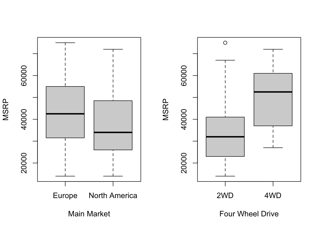
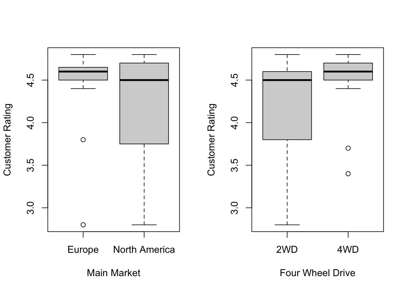
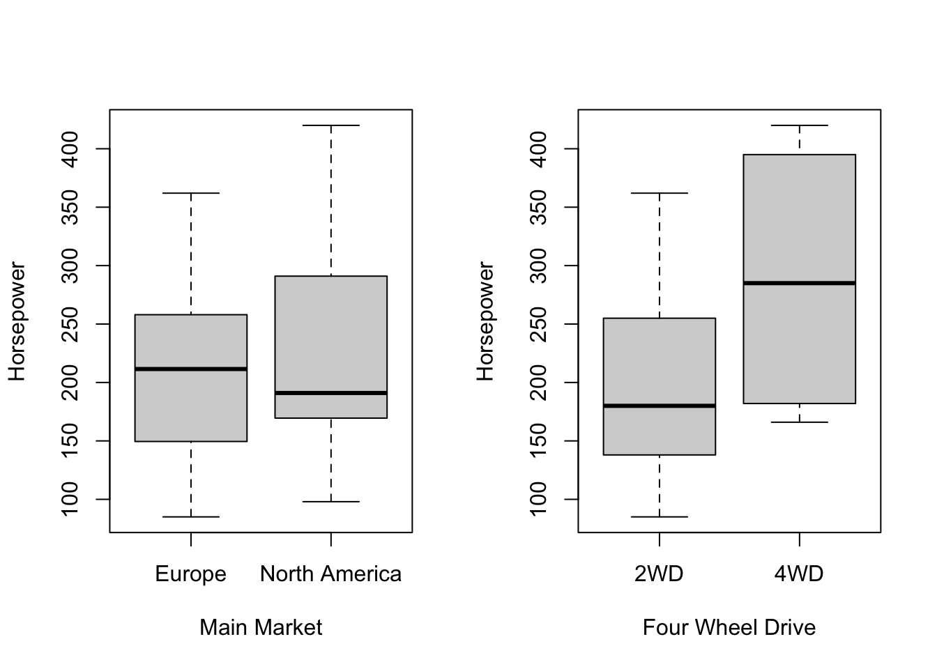
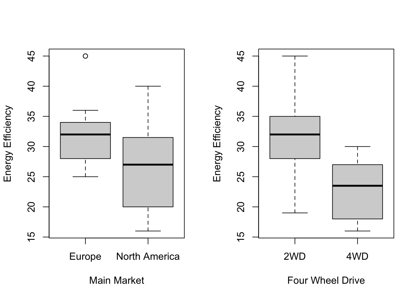
Scatterplots show how pricing and performance metrics vary across markets.
# Set up the plotting area to accommodate multiple plots
par(mfrow = c(1, 2))  # 4 rows, 2 columns layout

# Scatterplot: MSRP vs Customer Rating, colored by Main Market
plot(car_data_clean$`Customer Rating`, car_data_clean$`MSRP (USD)`,
     col = car_data_clean$`Main Market`,
     xlab = "Customer Rating", ylab = "MSRP", pch = 19)
legend("topleft", legend = levels(car_data_clean$`Main Market`), col = 1:2, pch = 19)

# Scatterplot: MSRP vs Customer Rating, colored by Four Wheel Drive
plot(car_data_clean$`Customer Rating`, car_data_clean$`MSRP (USD)`,
     col = car_data_clean$Four_Wheel_Drive,
     xlab = "Customer Rating", ylab = "MSRP", pch = 19)
legend("topleft", legend = levels(car_data_clean$Four_Wheel_Drive), col = 1:2, pch = 19)
# Scatterplot: MSRP vs Horsepower, colored by Main Market
plot(car_data_clean$Horsepower, car_data_clean$`MSRP (USD)`,
     col = car_data_clean$`Main Market`,
     xlab = "Horsepower", ylab = "MSRP", pch = 19)
legend("topleft", legend = levels(car_data_clean$`Main Market`), col = 1:2, pch = 19)

# Scatterplot: MSRP vs Horsepower, colored by Four Wheel Drive
plot(car_data_clean$Horsepower, car_data_clean$`MSRP (USD)`,
     col = car_data_clean$Four_Wheel_Drive,
     xlab = "Horsepower", ylab = "MSRP", pch = 19)
legend("topleft", legend = levels(car_data_clean$Four_Wheel_Drive), col = 1:2, pch = 19)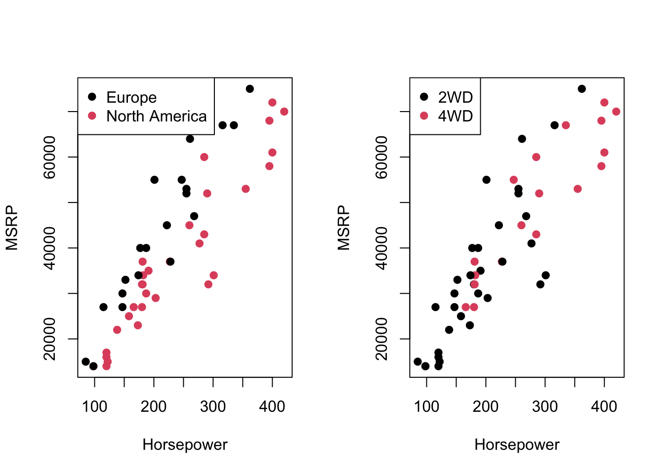
# Scatterplot: MSRP vs Energy Efficiency, colored by Main Market
plot(car_data_clean$`Energy Efficiency (MPG)`, car_data_clean$`MSRP (USD)`,
     col = car_data_clean$`Main Market`,
     xlab = "Energy Efficiency (MPG)", ylab = "MSRP", pch = 19)
legend("topright", legend = levels(car_data_clean$`Main Market`), col = 1:2, pch = 19)

# Scatterplot: MSRP vs Energy Efficiency, colored by Four Wheel Drive
plot(car_data_clean$`Energy Efficiency (MPG)`, car_data_clean$`MSRP (USD)`,
     col = car_data_clean$Four_Wheel_Drive,
     xlab = "Energy Efficiency (MPG)", ylab = "MSRP", pch = 19)
legend("topright", legend = levels(car_data_clean$Four_Wheel_Drive), col = 1:2, pch = 19)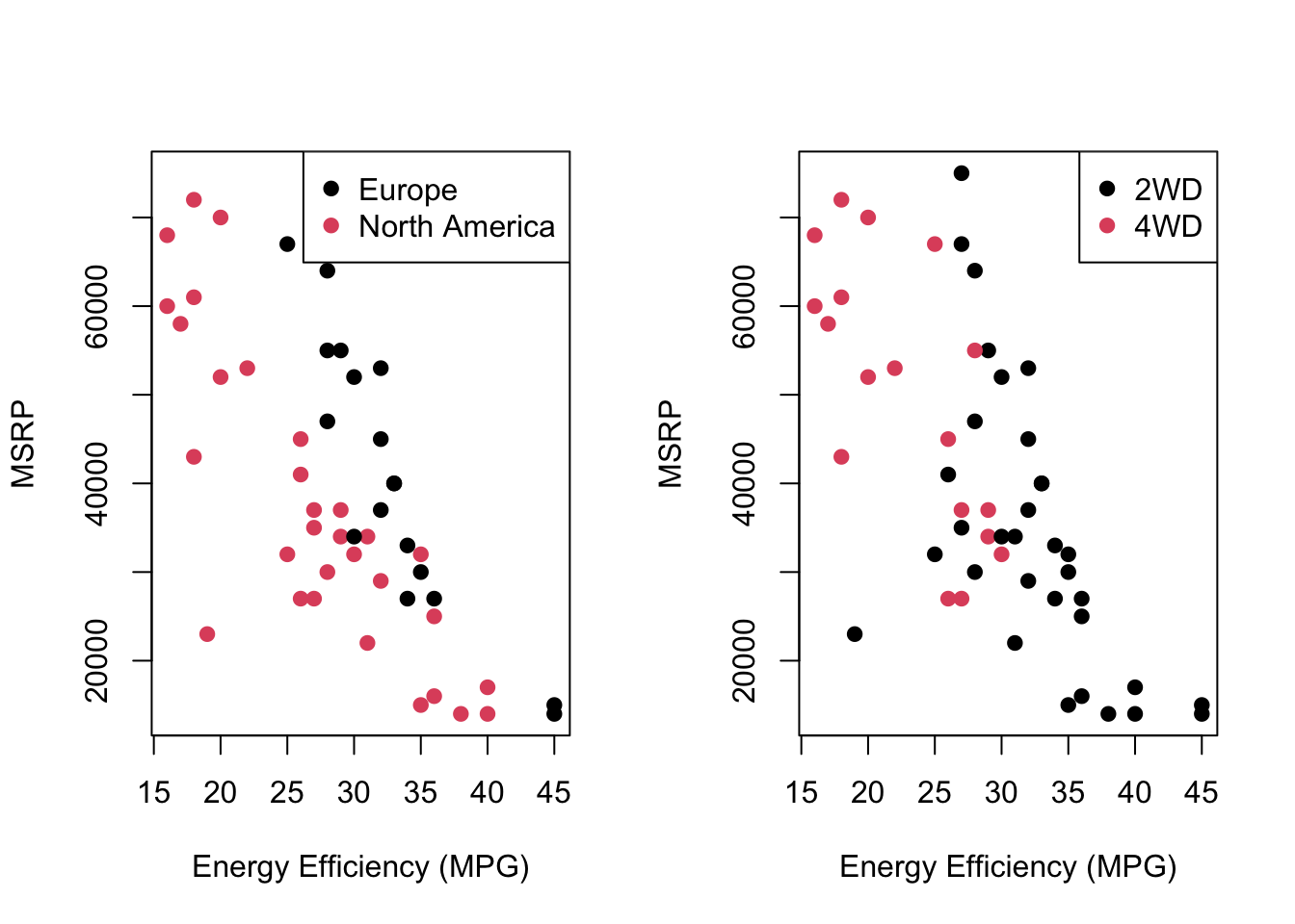
# Scatterplot: MSRP vs Customer Rating, colored by Main Market
plot(car_data_clean$`Customer Rating`, car_data_clean$`MSRP (USD)`,
     col = car_data_clean$`Main Market`,
     xlab = "Customer Rating", ylab = "MSRP", pch = 19)
legend("topleft", legend = levels(car_data_clean$`Main Market`), col = 1:2, pch = 19)

# Scatterplot: MSRP vs Customer Rating, colored by Four Wheel Drive
plot(car_data_clean$`Customer Rating`, car_data_clean$`MSRP (USD)`,
     col = car_data_clean$Four_Wheel_Drive,
     xlab = "Customer Rating", ylab = "MSRP", pch = 19)
legend("topleft", legend = levels(car_data_clean$Four_Wheel_Drive), col = 1:2, pch = 19)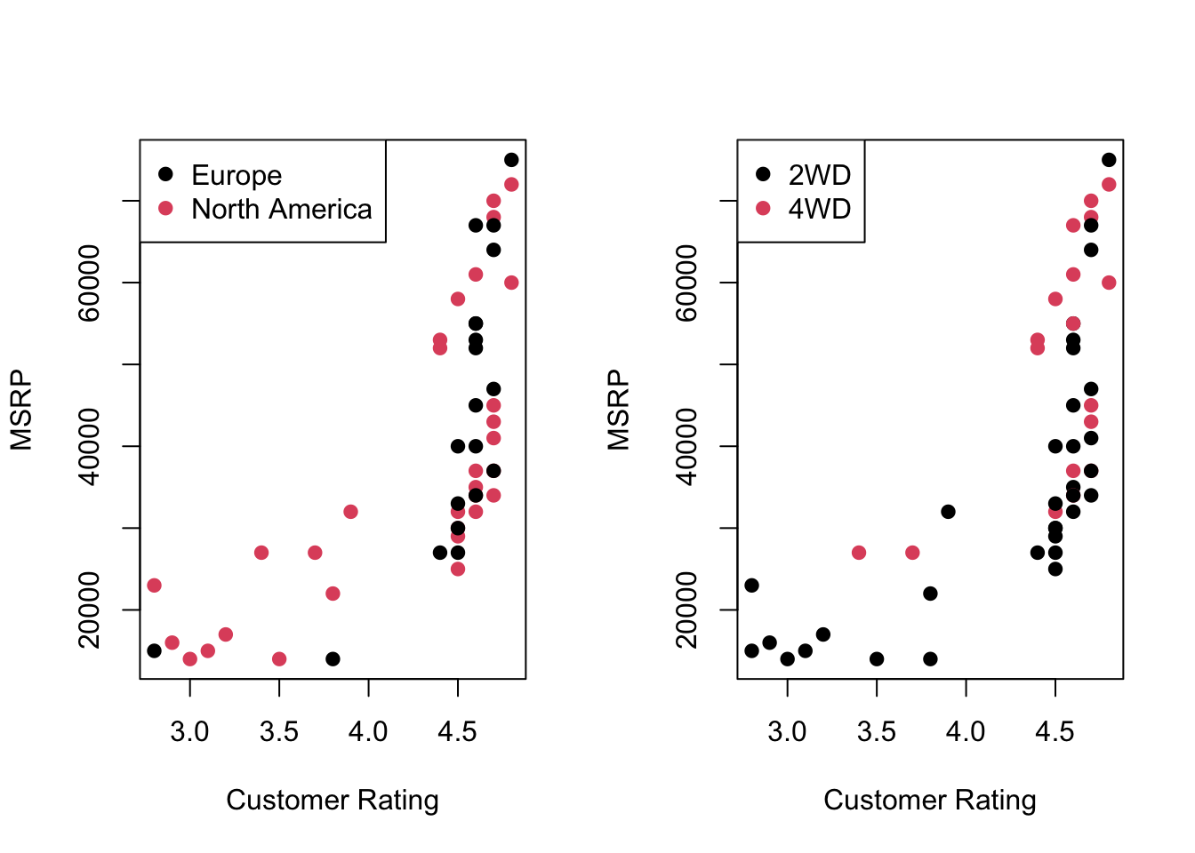
10.4 Statistical Modeling
To analyze the impact of customer satisfaction, performance metrics, and market-specific factors on vehicle pricing (MSRP), we first need to hot-code the North America Market variable. After encoding this variable, we fit a multiple linear regression model that includes Customer Rating, Energy Efficiency (MPG), Horsepower, and interaction terms for Horsepower and Four_Wheel_Drive with the North America Market.
Hot-Encoding North America Market
We create a new binary variable North America Market that takes the value 1 if the vehicle is sold in North America, and 0 otherwise (Europe). This binary encoding allows us to assess how market-specific factors influence vehicle pricing.
Fitting the Regression Model
With the North America Market variable encoded, we proceed to fit a multiple regression model that incorporates the key factors affecting MSRP and their interactions with the North American market.
Call:
lm(formula = `MSRP (USD)` ~ `Customer Rating` + `Energy Efficiency (MPG)` +
    Horsepower + Horsepower:`North America Market` + Four_Wheel_Drive:`North America Market`,
    data = car_data_clean)

Residuals:
     Min       1Q   Median       3Q      Max
-10660.6  -2431.3    137.7   2554.1  11210.7

Coefficients:
                                            Estimate Std. Error t value
(Intercept)                                 3452.689  10015.106   0.345
`Customer Rating`                           3648.499   1553.654   2.348
`Energy Efficiency (MPG)`                   -382.447    197.904  -1.932
Horsepower                                   172.361     15.359  11.222
Horsepower:`North America Market`            -61.933      8.329  -7.436
`North America Market`:Four_Wheel_Drive4WD  5493.988   2288.221   2.401
                                           Pr(>|t|)
(Intercept)                                  0.7319
`Customer Rating`                            0.0233 *
`Energy Efficiency (MPG)`                    0.0596 .
Horsepower                                 1.24e-14 ***
Horsepower:`North America Market`          2.31e-09 ***
`North America Market`:Four_Wheel_Drive4WD   0.0205 *
---
Signif. codes:  0 '***' 0.001 '**' 0.01 '*' 0.05 '.' 0.1 ' ' 1

Residual standard error: 4879 on 45 degrees of freedom
Multiple R-squared:  0.9283,    Adjusted R-squared:  0.9203
F-statistic: 116.5 on 5 and 45 DF,  p-value: < 2.2e-16
The fitted model includes: - Customer Rating: Influence of customer satisfaction on MSRP. - Energy Efficiency (MPG): Impact of fuel efficiency on vehicle pricing. - Horsepower: Effect of engine power on MSRP. - Interaction Terms: How the impact of horsepower and four-wheel drive on pricing changes in the North American market compared to other regions.
Mathematical Representation of the Model
The regression model, including all the variables and interaction terms, can be written as the following equation:
\[ \begin{aligned} \text{MSRP} = & \, \beta_0 + \beta_1 \cdot \text{Customer Rating} + \beta_2 \cdot \text{Energy Efficiency (MPG)} \\ & + \beta_3 \cdot \text{Horsepower} + \beta_4 \cdot (\text{Horsepower} \times \text{North America Market}) \\ & + \beta_5 \cdot (\text{Four Wheel Drive} \times \text{North America Market}) + \epsilon \end{aligned} \]
Where:
- \(\beta_0\) is the intercept.
-
\(\beta_1\) is the coefficient for
Customer Rating. -
\(\beta_2\) is the coefficient for
Energy Efficiency (MPG). -
\(\beta_3\) is the coefficient for
Horsepower. -
\(\beta_4\) is the coefficient for the interaction between
HorsepowerandNorth America Market. -
\(\beta_5\) is the coefficient for the interaction between
Four Wheel DriveandNorth America Market. - \(\epsilon\) represents the residual (error term).
This equation models how customer satisfaction, performance metrics like horsepower, and interaction effects related to the North American market influence vehicle pricing (MSRP). The interaction terms allow us to capture how the effects of horsepower and four-wheel drive on pricing may vary depending on the market region.
10.5 Model Interpretation
The coefficients reveal important insights:
- Customer Rating: Each 1-point increase in customer satisfaction raises MSRP by approximately $3,648, indicating that customer satisfaction significantly impacts pricing.
- Energy Efficiency: A 1-MPG increase slightly reduces MSRP by $382, suggesting that fuel efficiency may be less valued in pricing decisions.
- Horsepower: For each additional unit of horsepower, MSRP increases by $172, confirming that performance metrics like horsepower drive higher vehicle pricing.
- Interaction Terms: Horsepower has a smaller effect on pricing in the North American market, while four-wheel-drive vehicles command a higher premium in North America compared to other regions.
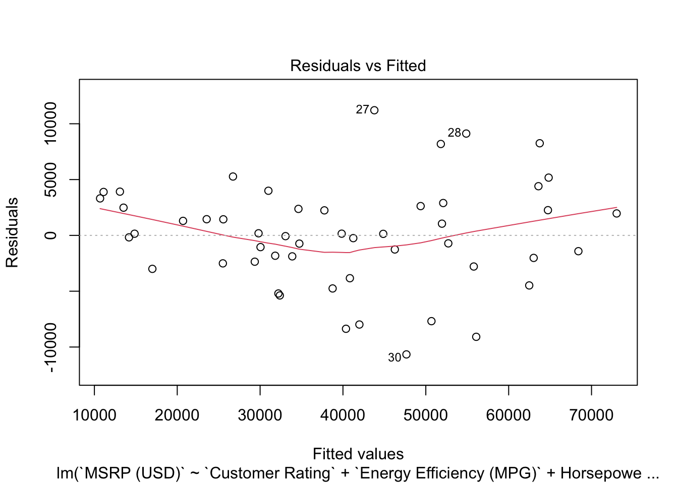
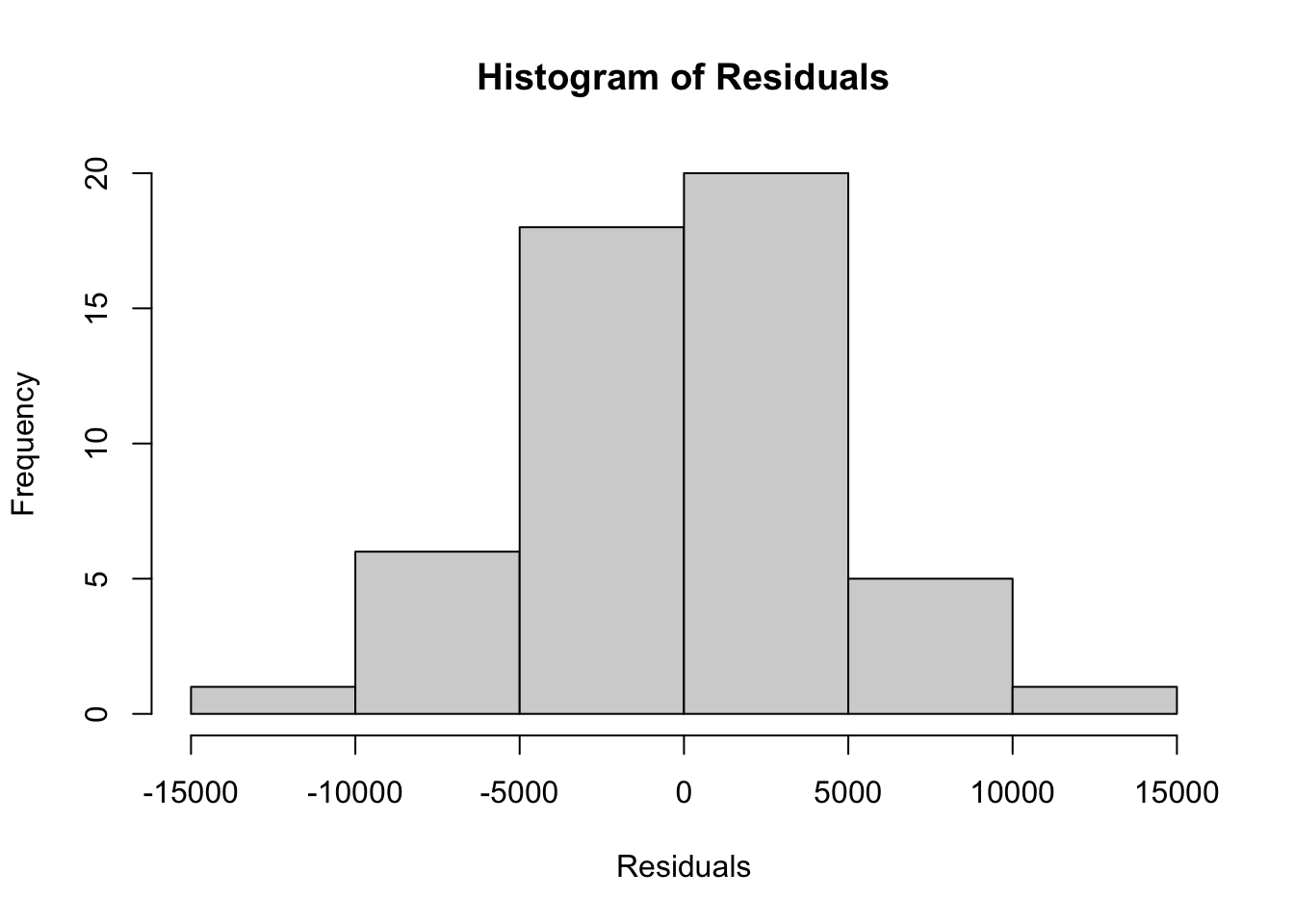
10.6 Model Diagnostics
We use residual plots and k-fold cross-validation to assess the model’s performance.
Loading required package: lattice
Attaching package: 'caret'The following objects are masked from 'package:DescTools':
MAE, RMSEThe following object is masked from 'package:purrr':
lifttrain_control <- trainControl(method = "cv", number = 5)
cv_model <- train(`MSRP (USD)` ~ `Customer Rating` + `Energy Efficiency (MPG)` + Horsepower +
Horsepower:`North America Market` + Four_Wheel_Drive:`North America Market`,
data = car_data_clean, method = "lm", trControl = train_control)
cv_modelLinear Regression
51 samples
5 predictor
No pre-processing
Resampling: Cross-Validated (5 fold)
Summary of sample sizes: 41, 39, 41, 41, 42
Resampling results:
RMSE Rsquared MAE
5052.881 0.9167011 4055.627
Tuning parameter 'intercept' was held constant at a value of TRUE10.7 Hypothesis Test: Does a 0.5 Increase in Customer Rating Lead to at Least $1000 Increase in MSRP?
To test the hypothesis, we will evaluate whether a 0.5 increase in customer satisfaction results in a price increase of at least $1000.
Hypotheses:
- \(H_0\): The increase in MSRP due to a 0.5 increase in Customer Rating is less than or equal to $1000.
- \(H_1\): The increase in MSRP due to a 0.5 increase in Customer Rating is greater than $1000.
Test Calculation:
- We extract the coefficient for
Customer Ratingfrom the model. - Calculate the expected price increase for a 0.5-point increase in customer satisfaction.
- Conduct a one-sided t-test to compare the expected increase to the $1000 threshold.
# Extract the coefficient and standard error for Customer Rating
coef_customer_rating <- coef(summary(model1))[2, 1]
se_customer_rating <- coef(summary(model1))[2,2]

# Calculate the expected increase in MSRP for a 0.5 increase in Customer Rating
expected_increase <- coef_customer_rating * 0.5

# Calculate the standard error for the expected increase
se_increase <- se_customer_rating * 0.5

# Perform the one-sided t-test
t_stat <- (expected_increase - 1000) / se_increase
p_value <- pt(t_stat, df = df.residual(model1), lower.tail = FALSE)

# Output the results
list(expected_increase = expected_increase, t_statistic = t_stat, p_value = p_value)
$expected_increase
[1] 1824.25
$t_statistic
[1] 1.061047
$p_value
[1] 0.1471652Interpretation of Results
- Expected Increase: The predicted increase in MSRP for a 0.5-point increase in customer rating is compared to the $1000 threshold.
- t-statistic: Indicates how many standard errors the predicted increase is from $1000.
- p-value: If the p-value is less than 0.05, we reject the null hypothesis and conclude that the increase in customer satisfaction will likely result in an increase in MSRP greater than $1000, justifying the investment.
10.8 Conclusion
In this chapter, we explored how vehicle pricing is influenced by performance metrics, market factors, and customer satisfaction. We fit a multiple regression model and performed a hypothesis test to determine whether a 0.5-point increase in customer satisfaction would result in an MSRP increase of at least $1000. The analysis shows that customer satisfaction significantly affects pricing, and the hypothesis test provides insights into whether the new feature justifies its cost.
10.9 Homework Assignment: Evaluating the Commercial Viability of a New Safety Feature
10.9.1 Objective
In this assignment, you will evaluate whether adding a new safety feature that increases the vehicle safety rating by 1 point is commercially viable, given that it increases production costs by $500. You will use multiple regression analysis to examine the relationship between safety rating, MSRP (Manufacturer’s Suggested Retail Price), and other relevant variables, and perform hypothesis testing to determine whether the expected price increase justifies the production cost.
10.9.2 Submission Instructions
Please follow these detailed instructions for completing and submitting your assignment. This assignment is to be conducted within the class assignment workspace provided to you. You will create an R Quarto document, incorporating code and analysis as demonstrated in the provided examples. Follow the structure provided in the example code and explanations to guide your analysis. Each required step should correspond to a separate section within your R Quarto document. Utilize the headings feature in Quarto to organize your document (# for main sections, ## for subsections). Once you have completed the analysis and are satisfied with your document, compile it into MS Word document and submit it as instructed.