19 Dealing with Endogeneity Bias
PRELIMINARY AND INCOMPLETE
In the realm of regression analysis, understanding the concept of endogeneity is crucial. Endogeneity occurs when an explanatory variable is correlated with the error term in a regression model, leading to biased and inconsistent estimates. Ignoring endogeneity in models can result in misleading inferences, which can have significant implications for decision-making in business and economics. This chapter delves into the sources of endogeneity, its consequences, and how to address it using the Instrumental Variables (IV) approach and Two-Stage Least Squares (2SLS) method.
19.1 Chapter Goals
Upon concluding this chapter, readers will be able to:
- Define endogeneity and distinguish it from exogeneity in the context of regression models
- Understand common sources of endogeneity, including omitted variables, simultaneity, measurement error, and the ratio problem, and explain how they affect regression analysis
- Apply visual inspection, correlation analysis, and statistical tests to diagnose the presence of endogeneity in regression models
- Analyze the impact of endogeneity on regression estimates, particularly how it introduces bias and inconsistency, and understand its implications for model validity
- Evaluate the relevance and exogeneity of potential instrumental variables, determining whether they are suitable for addressing endogeneity in a given model
- Create an implementation of the Instrumental Variables (IV) approach and perform Two-Stage Least Squares (2SLS) regression to address endogeneity, using R or other statistical tools
- Evaluate the differences between Ordinary Least Squares (OLS) and IV estimates, interpreting the effectiveness of the IV approach in obtaining consistent and unbiased estimates
- Apply the knowledge of endogeneity to recognize scenarios where the complexity of the issue necessitates seeking assistance from econometric experts to ensure accurate model specification and interpretation
19.2 Understanding the Concept of Endogeneity
Endogeneity arises in a regression model when an explanatory variable is correlated with the error term. This correlation can stem from several sources, such as omitted variables, simultaneity, or measurement error. When endogeneity is present, the ordinary least squares (OLS) estimates become biased and inconsistent, making it difficult to draw reliable conclusions from the model.
19.2.1 How Endogeneity Differs from Exogeneity
- Exogeneity: An explanatory variable is exogenous when it is not correlated with the error term in the regression model. This lack of correlation ensures that the estimates of the coefficients are unbiased and consistent.
- Endogeneity: An explanatory variable is endogenous when it is correlated with the error term. This correlation introduces bias in the coefficient estimates, leading to inconsistent and unreliable results.
19.2.2 Examples of Endogeneity in Real-World Scenarios
- Omitted Variables: Consider a study examining the effect of education on earnings. If the model omits variables like work experience or innate ability, which are correlated with both education and earnings, the estimates of the effect of education on earnings will be biased due to the omitted variable bias.
- Simultaneity: In supply and demand models, price and quantity are determined simultaneously. This simultaneity causes endogeneity because the quantity demanded influences the price, and the price influences the quantity demanded.
- Measurement Error: When studying the impact of advertising on sales, if the advertising expenditure is measured with error, this measurement error can lead to endogeneity, as the observed advertising variable is correlated with the error term in the regression model.
19.2.3 A Simulated Example
To illustrate the concept of endogeneity, we simulate data and visualize the impact of endogeneity on regression estimates.
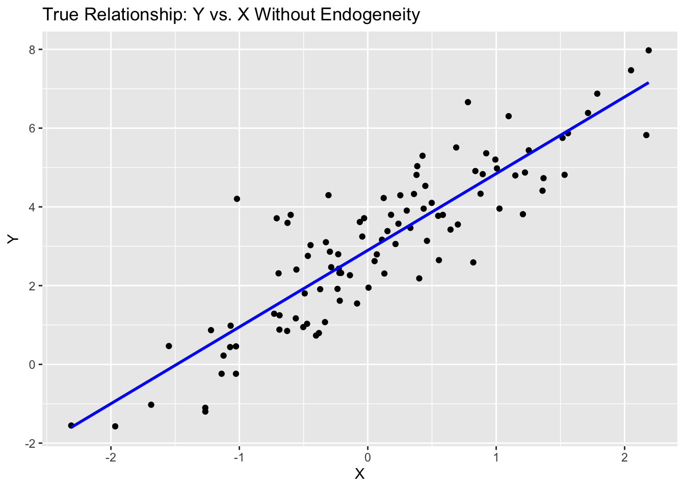
In this simulation, we generate data for 100 observations. The explanatory variable\(x\)is drawn from a standard normal distribution, and the error term\(e\)is normally distributed as well. The true model is specified as:
\[ y = 3 + 2x + e \]
Here is a scatter plot visualizing the true relationship:
To introduce endogeneity, we create an endogenous explanatory variable\(x_{\text{endogenous}}\)by adding a larger portion of the error term to\(x\):
\[ x_{\text{endogenous}} = x + 2e \]
This makes\(x_{\text{endogenous}}\)strongly correlated with the error term\(e\), thus violating the exogeneity assumption. We then fit an OLS model using\(x_{\text{endogenous}}\)as the explanatory variable:
Call:
lm(formula = y ~ x, data = data_endog)

Residuals:
    Min      1Q  Median      3Q     Max
-3.0847 -0.7808 -0.0678  0.7689  3.3049

Coefficients:
            Estimate Std. Error t value Pr(>|t|)
(Intercept)  3.16732    0.12697   24.95   <2e-16 ***
x            0.75433    0.06074   12.42   <2e-16 ***
---
Signif. codes:  0 '***' 0.001 '**' 0.01 '*' 0.05 '.' 0.1 ' ' 1

Residual standard error: 1.267 on 98 degrees of freedom
Multiple R-squared:  0.6115,    Adjusted R-squared:  0.6075
F-statistic: 154.2 on 1 and 98 DF,  p-value: < 2.2e-16
Note how the coefficient on\(x\)with endogeneity present differs from the true relationship. This can also be seen when we visualize the relationship between\(x_{\text{endogenous}}\)and\(y\).
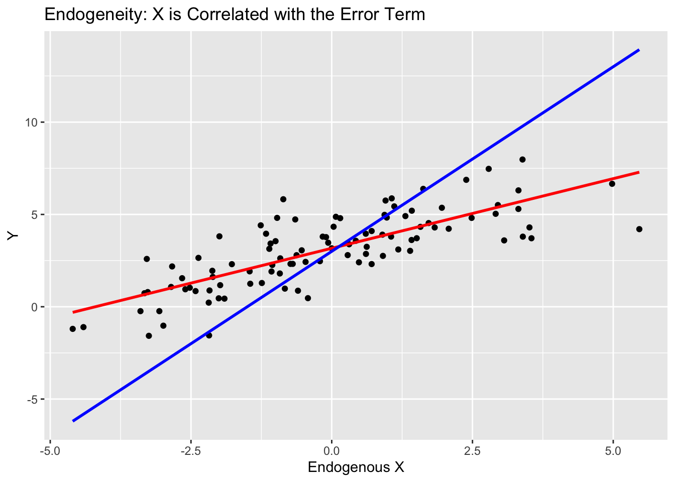
The scatter plot and fitted lines from the linear models highlight the bias introduced by endogeneity. The red line represents the OLS estimate, which is biased because\(x_{\text{endogenous}}\)is correlated with the error term. The blue line represents the true relationship between\(x\)and\(y\). This visualization illustrates how endogeneity can distort the true relationship between variables in a regression model, leading to misleading inferences.
In this chapter, we will discuss how to identify and correct for some common forms of endogeneity. We will discuss the use of instrumental variables. This is a big topic, and you may not feel fully comfortable conducting this analysis on your own by the end of this chapter. That’s okay. The important thing is to understand some of the common situations where this problem can occur and understand the implications on analysis. At that point, you can decide if it is time to seek help from an expert. In my opinion, that is a good outcome.
19.3 Identifying Sources of Endogeneity
Endogeneity is a common issue in regression analysis that can arise from several sources. Understanding and identifying these sources is crucial for developing accurate and reliable models. This section explores a few of the common sources of endogeneity: omitted variables, measurement error, simultaneity, and the ratio problem. Each of these sources can introduce bias and inconsistency into regression estimates, leading to misleading inferences and poor decision-making.
19.3.1 Omitted Variables
Omitted variable bias arises when a relevant variable is left out of the regression model, causing the included variables to capture the effect of the missing variable. This often happens in complex systems where many factors influence the outcome, and not all of these factors are observed or measured. To identify omitted variables, one should start with theoretical considerations, looking for variables that should logically affect the dependent variable but are not included in the model. For instance, in a model analyzing the effect of education on earnings, work experience is a crucial variable. If work experience is omitted and it is correlated with both education and earnings, the coefficient of education will capture part of the effect of work experience, leading to biased estimates. Another way to identify omitted variables is through robustness checks. By including potential omitted variables in the model and observing if the coefficients of the included variables change significantly, one can infer the presence of omitted variable bias. The implications of omitted variables are severe; if these variables are correlated with both the explanatory and dependent variables, the estimated coefficients will be biased and inconsistent, making the model unreliable for inference or prediction.
19.3.2 Measurement Error
Measurement error occurs when the variables included in the model contain inaccuracies. This error can be present in both the dependent and explanatory variables, leading to different types of biases. To identify measurement error, one can compare measured values with known benchmarks or repeated measurements. Statistical tests or instruments can also be employed to detect and correct for measurement error. For example, if a company measures advertising expenditure inaccurately and uses this variable to estimate its impact on sales, the resulting coefficient will be biased. Measurement error in the dependent variable typically increases the variance of the estimates, making them less precise. In contrast, measurement error in the explanatory variables leads to biased and inconsistent estimates. This is because the explanatory variables no longer provide an accurate representation of the true underlying factors affecting the dependent variable.
19.3.3 Simultaneity
Simultaneity arises when the dependent variable and one or more explanatory variables mutually influence each other, leading to endogeneity. This situation is common in economic models, such as supply and demand models, where price and quantity are determined simultaneously. In such cases, the quantity demanded influences the price, and the price influences the quantity demanded, causing endogeneity. To identify simultaneity, one should rely on theoretical knowledge and apply statistical tests such as the Wu-Hausman test. The implications of simultaneity are significant: it leads to biased and inconsistent estimates because the explanatory variable is determined simultaneously with the dependent variable. For example, in the housing market, the price of a house (dependent variable) and the demand for houses (explanatory variable) influence each other. If this simultaneity is not accounted for, the estimated effect of price on demand (or vice versa) will be biased, leading to incorrect conclusions about the market dynamics. Recognizing and addressing simultaneity is essential for developing accurate and reliable models in economics and business analysis.
19.3.4 The Ratio Problem
The ratio problem is a specific type of endogeneity that occurs when a ratio is used as an explanatory variable, and the denominator of the ratio is correlated with the error term. This can introduce bias because the denominator’s variations can affect both the ratio and the dependent variable. For instance, in a financial analysis, using the debt-to-income ratio as an explanatory variable can be problematic if the income (denominator) is correlated with the error term in the regression model. To identify the ratio problem, one should examine the components of the ratio and their potential correlations with the error term. Addressing this issue often involves using alternative modeling techniques, such as including the numerator and denominator as separate variables or employing instrumental variables that are not correlated with the error term.
Understanding and addressing these sources of endogeneity is critical for ensuring the validity and reliability of regression models. In the following sections, we will discuss various methods to detect and correct for endogeneity, helping analysts to make more accurate and informed decisions.
19.4 Identifying and Testing for Endogeneity
Identifying and testing for endogeneity is a critical step in regression analysis to ensure the accuracy and reliability of the estimated coefficients. Endogeneity can arise from various sources, such as omitted variables, measurement error, and simultaneity, and it can lead to biased and inconsistent estimates. This section outlines the procedures for identifying and testing for endogeneity, using the data simulated in Section 1 as an example.
19.4.1 Visual Inspection
Visual inspection is a preliminary step to identify potential endogeneity issues by examining the relationship between the explanatory variable and the dependent variable. It involves several techniques. First, scatter plots are used to plot the dependent variable against the explanatory variable, allowing for the visualization of their relationship. If the data points systematically deviate from the regression line, this may indicate that the explanatory variable is correlated with the error term, suggesting endogeneity. Adding a regression line to the scatter plot can further reveal deviations from the expected linear relationship. Significant deviations may indicate endogeneity, as they suggest that the explanatory variable is capturing some of the error term’s variance. Changes in the slope of the regression line when additional variables are included or excluded from the model can indicate omitted variable bias. If the slope changes significantly, it suggests that the excluded variables are correlated with both the dependent and explanatory variables, leading to endogeneity. Lastly, residual plots, which plot the residuals from the OLS regression model against the explanatory variable, can help detect patterns or trends. If the residuals show a systematic pattern, it suggests that the explanatory variable is correlated with the error term, indicating endogeneity.
However, visual inspection has limitations. One significant limitation is that the true residuals are not observable. Instead, we work with estimated residuals from the OLS model, which can only approximate the true residuals. This approximation can sometimes obscure the presence of endogeneity or falsely indicate its presence. Therefore, while visual inspection is a useful preliminary tool, it should not be solely relied upon for diagnosing endogeneity. More robust methods, such as correlation analysis and statistical tests, are necessary to confirm its presence.
19.4.2 Correlation Analysis
Correlation analysis involves checking for correlation between the explanatory variables and the error term. This can be done through residual analysis to detect potential endogeneity. If the explanatory variable is correlated with the residuals, it indicates that the explanatory variable is endogenous. However, like visual inspection, correlation analysis is limited by the fact that true residuals are not observable. We rely on estimated residuals from the OLS model, which may not perfectly reflect the true residuals. Despite this limitation, a significant correlation between the residuals and the explanatory variable suggests that the explanatory variable is correlated with the error term, indicating endogeneity.
19.4.3 Instrumental Variables (IV) Approach
The Instrumental Variables (IV) approach is a common method to address endogeneity.[^1 Note that IV is an umbrella term for several different methods. In this chapter we will focus on a common method called Two-Stage Least Squares (2SLS).] An instrumental variable provides a source of variation in the explanatory variable that is not correlated with the error term. For an instrument to be valid, it must meet two main criteria: relevance and exogeneity. Relevance means that the instrument must be correlated with the endogenous explanatory variable, while exogeneity means that the instrument must be uncorrelated with the error term in the regression model. The IV approach typically involves two stages. In the first stage, the endogenous variable is regressed on the instrument to obtain predicted values. In the second stage, these predicted values are used in place of the endogenous variable in the regression model. This helps isolate the variation in the explanatory variable that is not correlated with the error term, thus addressing the endogeneity problem.
19.4.4 Statistical Tests for Endogeneity
Testing for endogeneity is not straightforward because the true residuals from the relationship are not observable. Instead, we rely on estimated residuals, which can introduce uncertainty in the testing process. Despite this limitation, these statistical tests can be used to detect endogeneity in regression models:
- Two-Stage Least Squares Compares the coefficient estimates of Two-Stage Least Squares (2SLS) to OLS by estimating residuals of the true model.
- Wu-Hausman Test: Compares OLS and IV estimates to test for endogeneity. If the estimates differ significantly, it suggests the presence of endogeneity.
- Durbin-Wu-Hausman Test: A more general test for endogeneity that also compares OLS and IV estimates.
- Hausman Test: Compares the difference between the coefficients obtained from OLS and IV regressions to detect endogeneity. A significant difference indicates endogeneity.
In this chapter, we will focus on Two-Stage Least Squares. Thus, the next section presents an example where we will compare the coefficient estimates of 2SLS to OLS.
19.5 Section 4: Basic Comparison to 2SLS
To illustrate the comparison between Ordinary Least Squares (OLS) and Two-Stage Least Squares (2SLS) in addressing endogeneity, we simulate a model where the dependent variable \(Y\) is related to the explanatory variables \(X\) and \(Z_1\). The model is specified as follows:
\[Y = \alpha_0 + \alpha_1 X + \alpha_2 Z_1 + \epsilon\]
Here, \(\alpha_0\) is the intercept, \(\alpha_1\) and \(\alpha_2\) are the coefficients of the explanatory variables, and \(\epsilon\) is the residual term drawn from a standard normal distribution. The endogeneity arises because \(\epsilon\) is present in both the equation for \(X\) and \(Y\). The following are how \(X\) and \(Y\) are simulated:
The equation for \(X\) is: \[X = 0.5 \cdot Z_1 + 0.3 \cdot Z_2 + 0.4 \cdot Z_3 + 2 * \epsilon\]
The equation for \(Y\) is: \[Y = 1.5 \cdot X + 0.5 \cdot Z_1 + \epsilon\]
These equations simulate the relationships between the variables, where \(\epsilon\) is drawn from a standard normal distribution and is present in both equations, thus creating endogeneity in the model. Note that \(Z_2\) and \(Z_3\) are drawn from a standard normal distribution, and the coefficients in both equation are simply made up. The reason for simulating data this way is that by doing so, we know that endogeneity is a problem and that \(Z_2\) and \(Z_3\) are appropriate instrumental variables Instrumental variables (IV) are used in regression analysis to provide consistent estimates when the explanatory variables are correlated with the error term.
19.5.1 Testing for Endogeneity
The procedure to test for endogeneity involves several steps, starting with a first stage regression, calculating residuals, conducting a second stage regression, and finally testing the significance of the residuals.
Step 1: First Stage Regression
In the first stage, we regress the potentially endogenous variable \(X\) on the instruments \(Z_2\) and \(Z_3\), as well as any other exogenous variables \(Z_1\), i.e.
\[X = \delta_0 + \delta_1 Z_1 + \delta_2 Z_2 + \delta_3 Z_3 + V\]
This helps us understand the relationship between\(X\)and the instruments and derive the residuals\(V\).
Call:
lm(formula = X ~ Z1 + Z2 + Z3)

Residuals:
     Min       1Q   Median       3Q      Max
-2.49138 -0.65392  0.05664  0.67033  2.53210

Coefficients:
            Estimate Std. Error t value Pr(>|t|)
(Intercept) -0.01933    0.10734  -0.180 0.857501
Z1           0.44455    0.11688   3.804 0.000251 ***
Z2           0.34622    0.10946   3.163 0.002091 **
Z3           0.34261    0.11223   3.053 0.002933 **
---
Signif. codes:  0 '***' 0.001 '**' 0.01 '*' 0.05 '.' 0.1 ' ' 1

Residual standard error: 1.052 on 96 degrees of freedom
Multiple R-squared:  0.2417,    Adjusted R-squared:  0.218
F-statistic:  10.2 on 3 and 96 DF,  p-value: 6.818e-06
In this step, we use lm(X ~ Z1 + Z2 + Z3) to perform the first stage regression and summarize the results. Note that in this step, we must check that the at least one of coefficients of \(Z_2\) or \(Z_3\) is significant. If it is not, then \(Z_2\) and \(Z_3\) may not be appropriate instrumental variables. Alternatively, we can use an f-test to check if \(Z_2\) and \(Z_3\) are jointly significant, in which case, they may be used together as instrumental variables. Luckly, both coefficents are significant.
Step 2: Calculate Residuals
After the first stage regression, we derive the residuals,\(V\), from the regression of \(X\) on \(Z_1\), \(Z_2\), and \(Z_3\). These residuals represent the part of \(X\) that is not explained by the instruments.
We extract the residuals from the first stage regression ,\(V\), using residuals(first_stage) and store them in V_hat.
19.5.1.1 Step 3: Second Stage Regression
In the second stage, we regress the dependent variable \(Y\) on \(X\), \(Z_1\), and the residuals \(\hat{V}\) from the first stage, i.e.
\[Y = \beta_0 + \beta_1 X + \beta_2 Z_1 + \gamma V + \epsilon\]
This allows us to test the significance of \(\hat{V}\) and determine if \(X\) is endogenous.
Call:
lm(formula = Y ~ X + Z1 + V_hat)

Residuals:
      Min        1Q    Median        3Q       Max
-0.166682 -0.046258 -0.005634  0.048103  0.196955

Coefficients:
             Estimate Std. Error t value Pr(>|t|)
(Intercept) -0.031800   0.007047  -4.513 1.81e-05 ***
X            1.488212   0.014980  99.345  < 2e-16 ***
Z1           0.454322   0.009594  47.356  < 2e-16 ***
V_hat        1.011788   0.016453  61.495  < 2e-16 ***
---
Signif. codes:  0 '***' 0.001 '**' 0.01 '*' 0.05 '.' 0.1 ' ' 1

Residual standard error: 0.07011 on 96 degrees of freedom
Multiple R-squared:  0.9994,    Adjusted R-squared:  0.9994
F-statistic: 5.411e+04 on 3 and 96 DF,  p-value: < 2.2e-16
In this step, we perform the second stage regression using lm(Y ~ X + Z1 + V_hat) and summarize the results.
Step 4: Test Significance
We test the significance of the coefficient on \(\hat{V}\) in the second stage regression. If this coefficient is significantly different from zero, it suggests that \(X\) is endogenous.
t test of coefficients:

              Estimate Std. Error  t value  Pr(>|t|)
(Intercept) -0.0317998  0.0071008  -4.4783 2.074e-05 ***
X            1.4882118  0.0146908 101.3026 < 2.2e-16 ***
Z1           0.4543216  0.0095893  47.3781 < 2.2e-16 ***
V_hat        1.0117882  0.0162338  62.3258 < 2.2e-16 ***
---
Signif. codes:  0 '***' 0.001 '**' 0.01 '*' 0.05 '.' 0.1 ' ' 1
We use coeftest with robust standard errors to test the significance of the coefficients in the second stage regression. The robust standard errors are computed using vcovHC(second_stage, type = "HC0").
As expected, the coefficient on \(\hat{V}\) (V_hat) is highly significant, which indicates that \(X\) is indeed an endogenous explanatory variable.
19.6 Dealing with Endogeneity
When you have determined that endogeneity is present in your regression model, there are several steps you can take to address it. Initially, you should attempt to eliminate endogeneity by including all relevant variables, improving measurement accuracy, and considering model specification changes. However, if these efforts do not resolve the issue, the next step is to use Instrumental Variables (IV).
19.6.1 Definition of Instrumental Variables (IV)
Instrumental variables (IV) are used in regression analysis to provide consistent estimates when the explanatory variables are correlated with the error term. This correlation can lead to endogeneity, causing biased and inconsistent estimates in Ordinary Least Squares (OLS) regression. IV’s help to isolate the variation in the explanatory variable that is not correlated with the error term, thereby addressing the endogeneity problem.
19.6.2 Conditions for a Valid Instrument
For an instrument to be valid, it must satisfy two key conditions:
Relevance: The instrument must be correlated with the endogenous regressor, meaning it should have a significant relationship with the variable it is intended to replace or adjust.
Exogeneity: The instrument must be uncorrelated with the residuals in the regression model. This ensures that the instrument does not introduce additional bias into the model.
19.6.3 Examples of Potential Instruments
Identifying valid instruments can be challenging, but some common sources include:
Historical Data: Using lagged values or past data that influence the endogenous regressor but not the dependent variable directly.
External Variables: Finding variables outside the model that affect the endogenous regressor but are uncorrelated with the error term. For example, weather conditions can be used as an instrument for agricultural output when studying the effect of agricultural output on economic growth.
19.6.4 Finding and Testing for Valid Instruments
Selecting valid instruments can be challenging. Effective strategies for selecting instruments involve both theoretical understanding and empirical testing. One common approach is to use historical data or lagged variables that influence the endogenous regressor but not the dependent variable directly. For instance, in economic models, past values of an economic indicator can serve as instruments for current values if they affect the regressor but not the dependent variable. Another strategy is to find external variables that theory predicts are correlated with the endogenous regressor but are uncorrelated with the error term. For example, weather conditions can be an instrument for agricultural output when studying the effect of agricultural output on economic growth, as weather affects crop yields but not economic growth directly.
To ensure that the instrument is relevant, we can use the F-statistic in the first stage of 2SLS (Two-Stage Least Squares) regression. A high F-statistic indicates that the instrument is strongly correlated with the endogenous regressor. While the ivreg() function calculates this F-statistic for us, it is helpful to understand how to perform this calculation manually.
19.6.5 Checking for Relevance
Later in this chapter, we will use the ivreg() function to estimate the two-stage least squares (2SLS) estimate for our example model. However, for now, we will continue to perform the estimation manually. This approach has the added benefit of clarifying why this method is referred to as two-stage least squares.
We will begin by reviewing the first-stage regression using our simulated example, specifically:
\[ X = \delta_0 + \delta_1 Z_1 + \delta_2 Z_2 + \delta_3 Z_3 + V \]
This can be implemented in R as follows:
Call:
lm(formula = X ~ Z1 + Z2 + Z3)

Residuals:
     Min       1Q   Median       3Q      Max
-2.49138 -0.65392  0.05664  0.67033  2.53210

Coefficients:
            Estimate Std. Error t value Pr(>|t|)
(Intercept) -0.01933    0.10734  -0.180 0.857501
Z1           0.44455    0.11688   3.804 0.000251 ***
Z2           0.34622    0.10946   3.163 0.002091 **
Z3           0.34261    0.11223   3.053 0.002933 **
---
Signif. codes:  0 '***' 0.001 '**' 0.01 '*' 0.05 '.' 0.1 ' ' 1

Residual standard error: 1.052 on 96 degrees of freedom
Multiple R-squared:  0.2417,    Adjusted R-squared:  0.218
F-statistic:  10.2 on 3 and 96 DF,  p-value: 6.818e-06
Note that the instruments \(Z_1\) and \(Z_2\) are both individually significant, which indicates that they satisfy the relevance condition. If both had been insignificant, we could test for joint significance using an F-test, as shown below:
| Res.Df | RSS | Df | Sum of Sq | F | Pr(>F) |
|---|---|---|---|---|---|
| 98 | 128 | ||||
| 96 | 106 | 2 | 21.9 | 9.9 | 0.000123 |
Given that \(Z_1\) and \(Z_2\) are both individually significant, it is not surprising that the F-test statistic from the test above is also significant. This is important because it ensures the instrumental variables are strongly correlated with the endogenous regressor. If the instruments are weak (i.e., not significant), the resulting 2SLS estimates may not correct for endogeneity of \(X\), leading to unreliable conclusions about the relationships in the model. In essence, strong instruments are necessary to ensure that the method correctly isolates the exogenous variation needed for valid inference.
19.6.6 Checcking for relevence
Latter in the chapter we will use the ivreg() function to estimate the two stage least squares estimate of or example model.
But for now we will continue to estimate the procedure by hand. This has the added benifit of making clear why this method is called two stage least squares
We will estimate review the first stage regression using our simulated example, i.e. \(X = \delta_0 + \delta_1 Z_1 + \delta_2 Z_2 + \delta_3 Z_3 + V\) or in R code
Call:
lm(formula = X ~ Z1 + Z2 + Z3)

Residuals:
     Min       1Q   Median       3Q      Max
-2.49138 -0.65392  0.05664  0.67033  2.53210

Coefficients:
            Estimate Std. Error t value Pr(>|t|)
(Intercept) -0.01933    0.10734  -0.180 0.857501
Z1           0.44455    0.11688   3.804 0.000251 ***
Z2           0.34622    0.10946   3.163 0.002091 **
Z3           0.34261    0.11223   3.053 0.002933 **
---
Signif. codes:  0 '***' 0.001 '**' 0.01 '*' 0.05 '.' 0.1 ' ' 1

Residual standard error: 1.052 on 96 degrees of freedom
Multiple R-squared:  0.2417,    Adjusted R-squared:  0.218
F-statistic:  10.2 on 3 and 96 DF,  p-value: 6.818e-06
Note that the instruments \(Z_1\) and \(Z_2\) are both individually significant, which indicates that they meet the criteria for relevance. If both had been insignificant, we could test for joint significance using an f-test, i.e.
| Res.Df | RSS | Df | Sum of Sq | F | Pr(>F) |
|---|---|---|---|---|---|
| 98 | 128 | ||||
| 96 | 106 | 2 | 21.9 | 9.9 | 0.000123 |
Given that \(Z_1\) and \(Z_2\) are both individually significant, it is not unexpected that we find that the test F-test statistic above is also significant.
19.6.7 Implementing the Two-Stage Least Squares in R
The ivreg() function from the AER package in R is used to implement the 2SLS approach. This function facilitates the estimation of the model with instrumental variables. The ivreg() function has a few corrections built in that make it superior to calculating the 2SLS from scratch, but it is still good practice to estimate and inspect the first stage equation. The following is an overview of the steps involved in estimating a 2SLS model.
Step-by-Step Procedure:
- Identify Potential Instruments: Choose variables that are theoretically sound and meet the conditions of relevance and exogeneity.
- Test for Instrument Relevance: Use statistical tests to ensure the instruments are strongly correlated with the endogenous regressor.
-
Implement the IV Model: Use appropriate R functions, such as
ivreg(), to estimate the model with instrumental variables. - Interpret the Results: Compare the IV estimates with OLS estimates to check for consistency and reliability. Look for significant differences that indicate the presence of endogeneity.
- Report Findings: Summarize the results, including the tests for instrument validity and the interpretation of the coefficients. Highlight the impact of addressing endogeneity on the model’s estimates.
Step 1. Identify Potential Instruments
In our simulated example, we can cheat We already know that \(Z_1\) and \(Z_2\) are strung instruments for \(X\). We will look at a more realistic example in the next chapter.
Step 2. Test for Instrument Relevance
We completed this step in an earlier section, but here is a review of the code needed. First, estimate and inspect the first stage equation:
Call:
lm(formula = X ~ Z1 + Z2 + Z3)

Residuals:
     Min       1Q   Median       3Q      Max
-2.49138 -0.65392  0.05664  0.67033  2.53210

Coefficients:
            Estimate Std. Error t value Pr(>|t|)
(Intercept) -0.01933    0.10734  -0.180 0.857501
Z1           0.44455    0.11688   3.804 0.000251 ***
Z2           0.34622    0.10946   3.163 0.002091 **
Z3           0.34261    0.11223   3.053 0.002933 **
---
Signif. codes:  0 '***' 0.001 '**' 0.01 '*' 0.05 '.' 0.1 ' ' 1

Residual standard error: 1.052 on 96 degrees of freedom
Multiple R-squared:  0.2417,    Adjusted R-squared:  0.218
F-statistic:  10.2 on 3 and 96 DF,  p-value: 6.818e-06
Then test the instruments for joint significance:
| Res.Df | RSS | Df | Sum of Sq | F | Pr(>F) |
|---|---|---|---|---|---|
| 98 | 128 | ||||
| 96 | 106 | 2 | 21.9 | 9.9 | 0.000123 |
Step 3. Implement the IV Model
After confirming the relevance of the instruments, we can proceed to estimate the 2SLS model using the ivreg() function from the AER package. The code below demonstrates how to do this:
Call:
ivreg(formula = Y ~ X + Z1 | Z2 + Z3)

Residuals:
     Min       1Q   Median       3Q      Max
-3.40373 -1.07738 -0.06513  0.98009  2.86443

Coefficients:
            Estimate Std. Error t value Pr(>|t|)
(Intercept)  -0.1430     0.2645  -0.541   0.5900
X             1.7935     0.6845   2.620   0.0102 *
Z1            1.6003     2.3236   0.689   0.4926

Diagnostic tests:
                      df1 df2 statistic p-value
Weak instruments (X)    2  97 7.083e+00 0.00135 **
Weak instruments (Z1)   2  97 9.280e-01 0.39900
Wu-Hausman              2  95 6.884e+30 < 2e-16 ***
Sargan                  0  NA        NA      NA
---
Signif. codes:  0 '***' 0.001 '**' 0.01 '*' 0.05 '.' 0.1 ' ' 1

Residual standard error: 1.388 on 97 degrees of freedom
Multiple R-Squared: 0.7659, Adjusted R-squared: 0.761
Wald test: 9.052 on 2 and 97 DF,  p-value: 0.0002487
The model is specified using ivreg(Y ~ X + Z1 | Z2 + Z3), which estimates a two-stage least squares (2SLS) model where \(Y\) is the dependent variable, \(X\) is the endogenous regressor, and \(Z_2\) and \(Z_3\) serve as instrumental variables. In this formula, the | operator distinguishes the endogenous regressor \(X\) from its instruments, \(Z_2\) and \(Z_3\).
After running the model, the output is summarized using summary(iv_model, diagnostics = TRUE). This function call provides a detailed summary of the estimated model, including not only the coefficients and their significance but also additional diagnostic tests. By setting diagnostics = TRUE, the summary includes tests for the validity of the instruments, such as the F-statistics from the first-stage regression, which assess instrument relevance, as well as over-identification tests and endogeneity tests to ensure that the instruments are valid and that \(X\) is correctly treated as endogenous.
The output from the ivreg() function can be summarized as follows. The residuals section provides a summary of the distribution of the residuals, which represent the differences between the observed and predicted values of \(Y\). The summary statistics include the minimum, first quartile (1Q), median, third quartile (3Q), and maximum residual values. These statistics are important for evaluating the spread and symmetry of the residuals, which in turn aids in diagnosing the model’s fit.
The coefficients table presents the estimated coefficients for the intercept, \(X\), and \(Z_1\), along with their standard errors, t-values, and p-values. The intercept reflects the predicted value of \(Y\) when all regressors are zero. The estimated coefficient for \(X\) is 1.7935 (SE = 0.6845), yielding a \(t\) value of 2.620, \(p\) = .0102, indicating that \(X\) is statistically significant at the .05 level. However, the coefficient for \(Z_1\), estimated at 1.6003, is not statistically significant, \(p\) = .4926.
The diagnostic tests included in the output assess the validity of the instruments and the overall suitability of the model. The test for weak instruments related to \(X\) (i.e., \(Z_2\) and \(Z_3\)) yields a p-value of .00135, suggesting that the instruments are strong and not weak. In contrast, the test for weak instruments related to \(Z_1\) shows a p-value of .39900, indicating potential weakness in the instruments for \(Z_1\). The Wu-Hausman test evaluates whether \(X\) is endogenous, with a very low p-value (\(< 2 \times 10^{-16}\)), strongly confirming the endogeneity of \(X\). The Sargan test, which typically assesses over-identification, is not applicable in this case, as the model is exactly identified (i.e., the number of instruments equals the number of endogenous regressors).
The residual standard error is reported as 1.388 with 97 degrees of freedom, providing a measure of the typical size of the residuals, where smaller values indicate a better fit. The multiple \(R^2\) value is .7659, meaning that approximately 76.59% of the variance in \(Y\) is explained by the model. The adjusted \(R^2\) value is .761, which accounts for the number of predictors and provides a more accurate measure of the model’s fit. Finally, the Wald test evaluates the joint significance of the coefficients, with a test statistic of 9.052 and a p-value of .0002487, suggesting that the coefficients are jointly significant, meaning at least one coefficient is significantly different from zero.
19.7 Conclusion
Endogeneity is a pervasive issue in regression analysis that, if left unaddressed, can lead to biased and inconsistent estimates, ultimately compromising the validity of the model and the conclusions drawn from it. This chapter has provided a comprehensive overview of endogeneity, its sources, and the significant implications it has for regression analysis. By understanding the mechanisms that lead to endogeneity, such as omitted variables, simultaneity, and measurement error, analysts can better diagnose and address these problems.
The chapter also explored various methods to detect and correct endogeneity, with a focus on the Instrumental Variables (IV) approach and Two-Stage Least Squares (2SLS) method. Through simulated examples, we illustrated how endogeneity distorts the relationship between variables and demonstrated the steps involved in applying IV techniques to mitigate this issue.
Ultimately, recognizing and correcting for endogeneity is essential for developing reliable models that can inform sound decision-making in business and economics. While the concepts and techniques discussed may initially seem complex, the key takeaway is the importance of identifying potential sources of endogeneity and applying appropriate methods, such as 2SLS, to ensure the accuracy and robustness of regression analysis. For those encountering complex cases, seeking assistance from experts in econometrics is advisable, as even small errors in addressing endogeneity can lead to significant misinterpretations of the data.