5 Introduction to Regression Analysis

PRELIMINARY AND INCOMPLETE

In this chapter, you will delve into the essential concepts and techniques of linear regression analysis. By the end, you will have gained a comprehensive understanding of how to build, interpret, and validate regression models, along with the ability to apply these skills in practical business scenarios. The following goals outline the key competencies you will develop as you work through the material.

5.1 Chapter Goals

Upon concluding this chapter, readers will be equipped with the skills to:

Understand the Fundamentals of Linear Regression: Grasp the basic concepts and components of a linear regression model.
Construct and Interpret Linear Regression Models: Develop and interpret linear regression models in R.
Assess the Validity of a Linear Regression Model: Evaluate goodness of fit and diagnose potential issues in a linear regression model.
Conduct a Thorough Exploratory Data Analysis (EDA): Perform EDA to explore relationships between variables.
Apply Diagnostic Checks to Ensure Model Assumptions are Met: Conduct diagnostic checks to validate the assumptions of linear regression.
Refine and Optimize Regression Models: Refine models and select the most appropriate one using criteria like adjusted $R^2$.
Visualize Regression Results Effectively: Create and enhance visual representations of regression results.
Utilize Regression Analysis for Informed Decision-Making: Apply regression techniques to inform data-driven decision-making.

5.2 What Is a Linear Regression Model?

Regression analysis is a statistical method used to examine the relationships between two or more variables. In business contexts, regression helps in understanding how changes in one variable are associated with changes in another. This is particularly useful for making predictions, identifying trends, and optimizing processes.

Regression is widely used in various business domains, including finance, marketing, and operations, to model relationships such as sales forecasting, risk assessment, and demand estimation.

The Basic Linear Regression Equation

A linear regression model is represented by the equation:

\[Y = \beta_0 + \beta_1X + \epsilon\]

Where:

$Y$ is the dependent variable (the outcome we are trying to predict).
$X$ is the independent variable (the predictor).
$\beta_0$ is the intercept, representing the expected value of $Y$ when $X = 0$.
$\beta_1$ is the slope, indicating the change in $Y$ for a one-unit change in $X$.
$\epsilon$ is the residual term, capturing the difference between the observed and predicted values.

Let’s consider an example using the mtcars dataset in R, where we model the relationship between miles per gallon (mpg) and car weight (wt).

# Example using mtcars dataset
model <- lm(mpg ~ wt, data = mtcars)
summary(model)


Call:
lm(formula = mpg ~ wt, data = mtcars)

Residuals:
    Min      1Q  Median      3Q     Max 
-4.5432 -2.3647 -0.1252  1.4096  6.8727 

Coefficients:
            Estimate Std. Error t value Pr(>|t|)    
(Intercept)  37.2851     1.8776  19.858  < 2e-16 ***
wt           -5.3445     0.5591  -9.559 1.29e-10 ***
---
Signif. codes:  0 '***' 0.001 '**' 0.01 '*' 0.05 '.' 0.1 ' ' 1

Residual standard error: 3.046 on 30 degrees of freedom
Multiple R-squared:  0.7528,    Adjusted R-squared:  0.7446 
F-statistic: 91.38 on 1 and 30 DF,  p-value: 1.294e-10

The code above fits a linear regression model to predict mpg based on wt. The summary function provides detailed output, including the estimated coefficients for the intercept ($\beta_0$) and slope ($\beta_1$). Here is the output represented as an equation:

\[\hat{mpg} = 37.285-5.344 \cdot wt\]

Visualizing the regression line helps in understanding the relationship between the variables. Below is a plot of car weight against miles per gallon, with the fitted regression line.

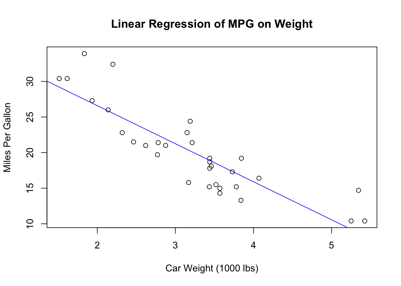
This plot shows how car weight affects fuel efficiency, with the blue line representing the best-fit line based on the linear regression model.

Linear regression is a versatile tool with numerous applications in business and economics, ranging from sales forecasting to risk assessment and demand estimation. For example, it can be used to predict future sales by analyzing historical data and market conditions, assess financial risks by modeling the relationship between economic indicators and asset prices, and estimate product demand based on factors like price, advertising, and consumer demographics. In the case of the mtcars dataset, linear regression can predict a car’s fuel efficiency based on its weight, a key consideration for automotive manufacturers and consumers. These are just a few examples of how linear regression provides valuable insights and supports data-driven decision-making in the business world.

5.3 Assumptions of Simple Linear Regression

After understanding the basic structure and applications of linear regression, it’s essential to consider the assumptions underlying the model. These assumptions play a critical role in ensuring that the results of the regression analysis are valid and reliable. Violating these assumptions can lead to misleading conclusions and poor decision-making. If the assumptions are not met, the model’s estimates can become biased, leading to incorrect conclusions.

Linearity:

The first assumption is that the relationship between the independent and dependent variables must be linear. In a linear regression model, the expectation is that as the independent variable changes, the dependent variable changes in a proportional and consistent manner. This linear relationship is fundamental to the accuracy of the model’s predictions. Visual inspections, such as scatterplots and residual plots, are commonly used to check for linearity.

Independence of Errors:

Another key assumption is that the residuals, or errors, are independent of each other. This means that the error for one observation should not be correlated with the error for another. Independence of errors is particularly important in time series data, where observations are collected over time. If the errors are correlated, it can indicate that important information has been omitted from the model, potentially leading to unreliable results.

Homoscedasticity:

Homoscedasticity refers to the assumption that the variance of residuals is constant across all levels of the independent variable. This means that the spread of the residuals should remain consistent regardless of the value of the predictor variable. When this assumption holds true, the model’s predictions are equally reliable across the entire range of the independent variable. If the variance of the residuals changes (a condition known as heteroscedasticity), it can indicate that the model does not equally capture the relationship between the variables at all levels.

Normality of Residuals:

The residuals of the model should follow a normal distribution. This assumption is important for making valid statistical inferences about the model’s coefficients. When residuals are normally distributed, the estimates of the model’s parameters are unbiased and have minimum variance, leading to more accurate predictions and confidence intervals.

Exogeneity of the Independent Variables:

Exogeneity is the assumption that the independent variables are not correlated with the error term. This means that the variation in the independent variable is assumed to be caused by factors outside the model and that these factors do not influence the dependent variable except through the independent variable. If this assumption is violated (a condition known as endogeneity), it can lead to biased and inconsistent estimates of the regression coefficients, rendering the model’s inferences invalid. Exogeneity is critical for establishing a causal relationship between the independent and dependent variables in the model.

No Perfect Multicollinearity (Relevant in Multiple Regression):

In the context of multiple regression, it is important that the independent variables are not perfectly correlated with each other. Perfect multicollinearity occurs when two or more independent variables in a model are perfectly correlated, making it impossible to isolate the individual effect of each predictor on the dependent variable. This assumption ensures that the model can distinguish between the effects of different predictors.

No Specification Bias:

The model must be correctly specified, which means including all relevant variables and using the correct functional form for the model. Omission of important variables or inclusion of irrelevant ones can lead to specification bias, which can distort the estimates of the regression coefficients. Correct specification is essential for ensuring that the model accurately captures the underlying relationship between the variables.

5.4 Interpreting Regression Output

Interpreting the coefficients in a regression model is essential for understanding the relationship between the independent and dependent variables and making informed business decisions. The following sections provide a detailed explanation of how to interpret these coefficients and the statistical measures associated with them.

The Slope and Intercept

The slope and intercept are the foundational components of a regression model. The intercept ($\beta_0$) represents the expected value of the dependent variable ($Y$) when the independent variable ($X$) is zero. In a business context, the intercept can be seen as the baseline level of $Y$ in the absence of $X$. For example, if you were modeling the relationship between advertising spend ($X$) and sales revenue ($Y$), the intercept would represent the sales revenue expected with no advertising spend.

The slope ($\beta_1$) indicates how much $Y$ is expected to change for a one-unit increase in $X$. This is crucial in business contexts as it quantifies the impact of $X$ on $Y$. Continuing with the previous example, the slope would tell you how much additional sales revenue is expected for each additional dollar spent on advertising.

Understanding the Regression Model Summary Output

A summery of the regression model can be obtained with summary(model). The regression model summary provides a detailed overview of the model’s performance and the statistical significance of its components, which is crucial for evaluating and interpreting the model’s results. The summary begins with a Call section, displaying the function used to fit the model—in this case, lm(formula = mpg ~ wt, data = mtcars)—indicating that the miles per gallon (mpg) is being predicted based on car weight (wt).

NecallNext, the Residuals section provides a summary of the residuals, which represent the differences between the observed and predicted values of the dependent variable. The summary includes the minimum, first quartile (1Q), median, third quartile (3Q), and maximum values of the residuals, showing the spread and distribution of these errors.

The Coefficients table is one of the most critical parts of the summary, listing the estimated coefficients for the intercept and the slope of the model. The Estimate column shows that the intercept ($\beta_0$) is 37.2851, which represents the expected mpg when the wt is zero. The slope ($\beta_1$) is -5.3445, indicating that for each unit increase in wt, the mpg is expected to decrease by 5.3445 units. The Std. Error column measures the precision of these estimates; smaller values indicate more reliable estimates. The t value assesses whether the coefficients are significantly different from zero, and the Pr(>|t|) column provides the p-values, which indicate the probability that the observed coefficients could occur by chance. In this case, both the intercept and slope have p-values close to zero, denoted by ***, signaling that they are highly statistically significant.

The Residual Standard Error (RSE), reported as 3.046, reflects the average distance between the actual data points and the regression line, with lower values indicating more accurate model predictions.

The Multiple R-squared value, 0.7528, indicates that approximately 75.28% of the variance in mpg is explained by wt. The Adjusted R-squared, slightly lower at 0.7446, accounts for the number of predictors in the model, providing a more accurate measure of the model’s goodness of fit.

Finally, the F-statistic of 91.38 tests the overall significance of the model, comparing it to a model with no predictors. The associated p-value of 1.294e-10 is very small, indicating that the model is statistically significant, meaning that wt is a meaningful predictor of mpg.

Confidence Intervals for Coefficients

Confidence intervals provide a range of values within which the true value of the regression coefficients is likely to fall, with a certain level of confidence (typically 95%). Constructing and interpreting confidence intervals for regression coefficients allows us to understand the uncertainty around our coefficient estimates.

confint(model)

                2.5 %    97.5 %
(Intercept) 33.450500 41.119753
wt          -6.486308 -4.202635

A narrow confidence interval suggests that the estimate is precise, whereas a wide interval indicates more uncertainty. If a confidence interval for a coefficient does not include zero, it implies that the coefficient is likely to be significantly different from zero, which is important for understanding the impact of the independent variable on the dependent variable.

Hypothesis Testing for Regression Coefficients

Hypothesis testing is used to determine whether the regression coefficients are statistically significant. The null hypothesis ($H_0$) typically states that the coefficient is equal to zero, meaning that the independent variable has no effect on the dependent variable. The alternative hypothesis ($H_A$) suggests that the coefficient is not zero.

The t-test evaluates these hypotheses by measuring how many standard deviations the estimated coefficient is away from zero. The p-value indicates the probability of observing the data if the null hypothesis is true. A small p-value (typically less than 0.05) suggests that the null hypothesis can be rejected, indicating that the coefficient is statistically significant.

summary(model)$coefficients

             Estimate Std. Error   t value     Pr(>|t|)
(Intercept) 37.285126   1.877627 19.857575 8.241799e-19
wt          -5.344472   0.559101 -9.559044 1.293959e-10

In business decision-making, a significant p-value implies that the corresponding independent variable has a meaningful impact on the dependent variable, justifying its inclusion in the model.

5.5 Conducting a Linear Regression in R: Workflow Overview

When conducting a linear regression in R, the process involves several key steps to ensure a thorough and accurate analysis:

Data Preparation: Load the data and handle missing values.
Exploratory Data Analysis (EDA): Perform exploratory analysis, including visualizing data with scatter plots to check for linear relationships.
Model Fitting: Fit the linear regression model using the lm() function and generate a detailed summary using summary().
Diagnostic Checks: Validate the model by checking residuals, assessing normality, and identifying any outliers or influential points.
Interpretation of Results: Examine the coefficients, determine the statistical significance, and evaluate the overall model fit.
Model Refinement and Reporting: Refine the model as needed and summarize the findings clearly, using visual aids to enhance understanding.

5.5.1 Step 1: Data Preparation

The first step in conducting a linear regression in R is to prepare your data. This involves loading the mtcars dataset into R and handling any missing values.

# Load the mtcars dataset
data(mtcars)

# Display the first few rows of the dataset
head(mtcars)

# Remove any rows with missing values (not needed for mtcars, but shown for completeness)
mtcars <- na.omit(mtcars)

Explanation of the code:
- data(mtcars): This loads the built-in mtcars dataset into the R environment. - head(mtcars): This function displays the first few rows of the mtcars dataset to help you inspect the data structure and contents. - na.omit(mtcars): Although the mtcars dataset does not have missing values, this function would remove any rows with missing values if they existed.

5.5.2 Step 2: Exploratory Data Analysis (EDA)

Before fitting the model, it’s essential to understand the relationships between the variables through exploratory data analysis. EDA involves generating summary statistics, creating visualizations such as scatterplots, and examining correlation matrices. One key aspect of EDA in linear regression is checking for linear relationships between the independent and dependent variables. A scatter plot is a useful tool for this purpose, allowing you to visually inspect whether a linear trend exists.

# Generate summary statistics for the dataset
summary(mtcars)

      mpg             cyl             disp             hp       
 Min.   :10.40   Min.   :4.000   Min.   : 71.1   Min.   : 52.0  
 1st Qu.:15.43   1st Qu.:4.000   1st Qu.:120.8   1st Qu.: 96.5  
 Median :19.20   Median :6.000   Median :196.3   Median :123.0  
 Mean   :20.09   Mean   :6.188   Mean   :230.7   Mean   :146.7  
 3rd Qu.:22.80   3rd Qu.:8.000   3rd Qu.:326.0   3rd Qu.:180.0  
 Max.   :33.90   Max.   :8.000   Max.   :472.0   Max.   :335.0  
      drat             wt             qsec             vs        
 Min.   :2.760   Min.   :1.513   Min.   :14.50   Min.   :0.0000  
 1st Qu.:3.080   1st Qu.:2.581   1st Qu.:16.89   1st Qu.:0.0000  
 Median :3.695   Median :3.325   Median :17.71   Median :0.0000  
 Mean   :3.597   Mean   :3.217   Mean   :17.85   Mean   :0.4375  
 3rd Qu.:3.920   3rd Qu.:3.610   3rd Qu.:18.90   3rd Qu.:1.0000  
 Max.   :4.930   Max.   :5.424   Max.   :22.90   Max.   :1.0000  
       am              gear            carb      
 Min.   :0.0000   Min.   :3.000   Min.   :1.000  
 1st Qu.:0.0000   1st Qu.:3.000   1st Qu.:2.000  
 Median :0.0000   Median :4.000   Median :2.000  
 Mean   :0.4062   Mean   :3.688   Mean   :2.812  
 3rd Qu.:1.0000   3rd Qu.:4.000   3rd Qu.:4.000  
 Max.   :1.0000   Max.   :5.000   Max.   :8.000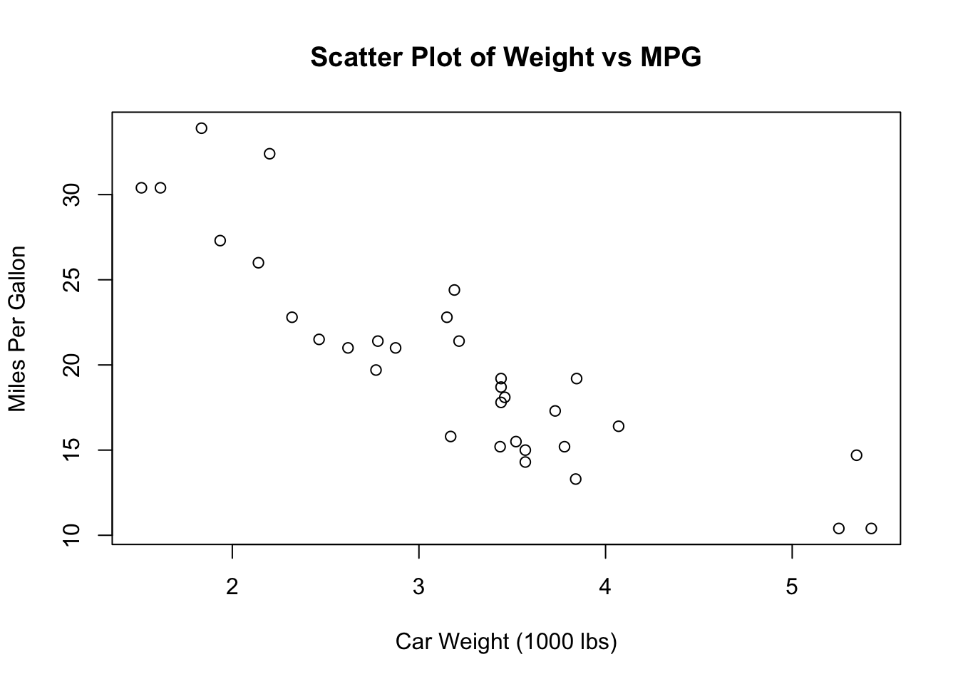

# Create a scatter plot to visualize the relationship between weight (wt) and miles per gallon (mpg)
plot(mtcars$wt, mtcars$mpg, main = "Scatter Plot of Weight vs MPG", 
     xlab = "Car Weight (1000 lbs)", ylab = "Miles Per Gallon")

Explanation of the code:
- summary(mtcars): This function provides summary statistics (such as mean, median, min, max) for each variable in the mtcars dataset, which helps in understanding the data distribution. - plot(mtcars$wt, mtcars$mpg): This function creates a scatter plot to visually inspect whether there is a linear relationship between car weight (wt) and miles per gallon (mpg). The main argument sets the title of the plot, while xlab and ylab label the x and y axes, respectively.

5.5.3 Step 3: Model Fitting

After completing the exploratory analysis, the next step is to fit the linear regression model. In R, this is done using the lm() function, where you specify mpg as the dependent variable (response) and wt as the independent variable (predictor). Once the model is fitted, you can use the summary() function to generate a detailed output that includes coefficient estimates, standard errors, t-values, p-values, and goodness-of-fit measures. This summary provides a comprehensive overview of the model’s performance, which is essential for evaluating its effectiveness.

# Fit the linear regression model
model <- lm(mpg ~ wt, data = mtcars)

# Generate a summary of the fitted model
summary(model)


Call:
lm(formula = mpg ~ wt, data = mtcars)

Residuals:
    Min      1Q  Median      3Q     Max 
-4.5432 -2.3647 -0.1252  1.4096  6.8727 

Coefficients:
            Estimate Std. Error t value Pr(>|t|)    
(Intercept)  37.2851     1.8776  19.858  < 2e-16 ***
wt           -5.3445     0.5591  -9.559 1.29e-10 ***
---
Signif. codes:  0 '***' 0.001 '**' 0.01 '*' 0.05 '.' 0.1 ' ' 1

Residual standard error: 3.046 on 30 degrees of freedom
Multiple R-squared:  0.7528,    Adjusted R-squared:  0.7446 
F-statistic: 91.38 on 1 and 30 DF,  p-value: 1.294e-10

Explanation of the code:
- lm(mpg ~ wt, data = mtcars): This function fits a linear regression model where mpg is the dependent variable and wt is the independent variable. The formula mpg ~ wt specifies this relationship. - summary(model): This function generates a detailed summary of the fitted model, including coefficient estimates, standard errors, t-values, p-values, and measures of goodness-of-fit like R-squared.

5.5.4 Step 4: Diagnostic Checks

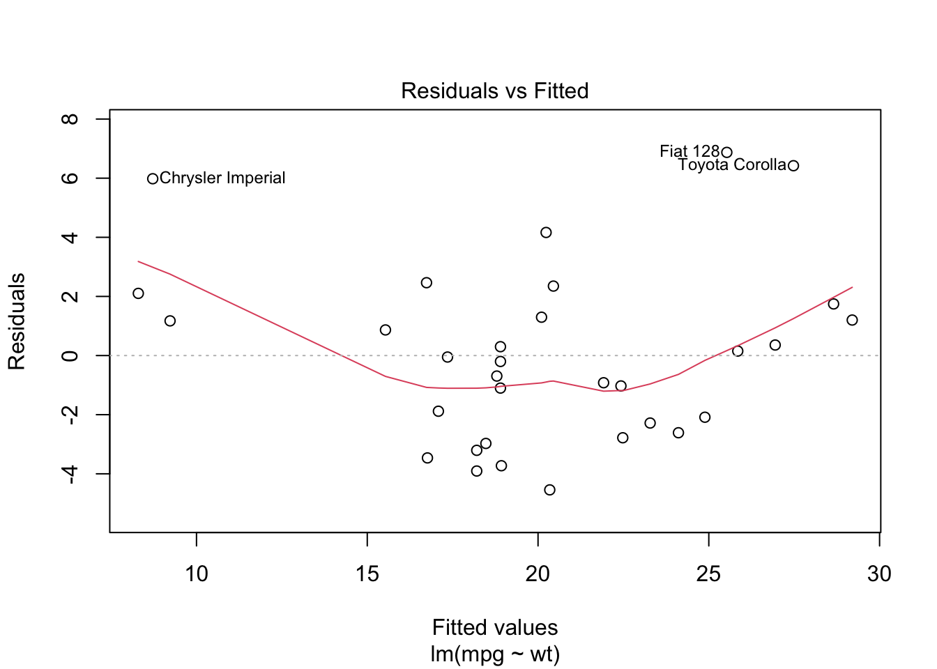
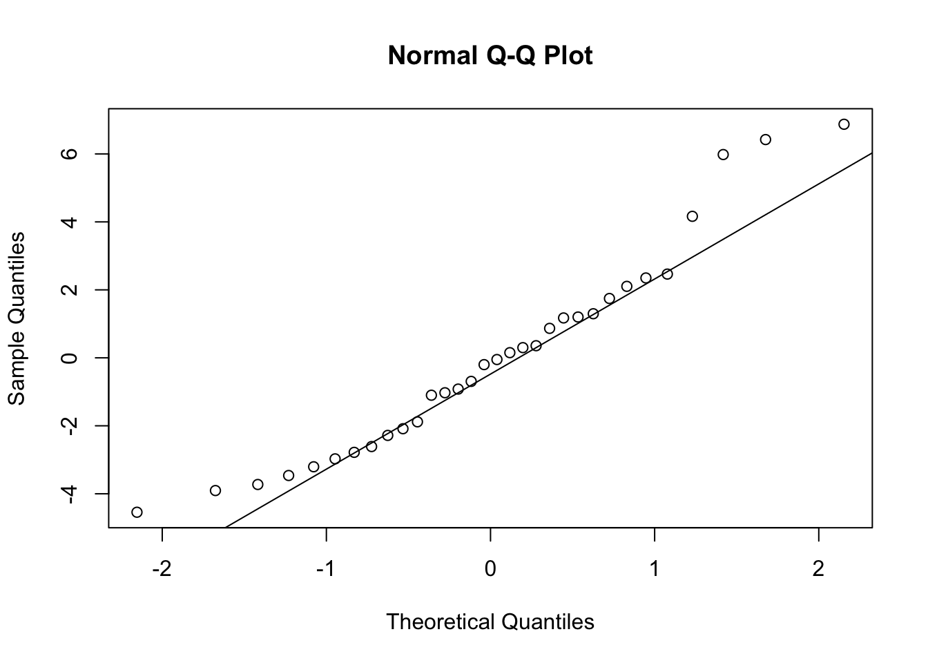
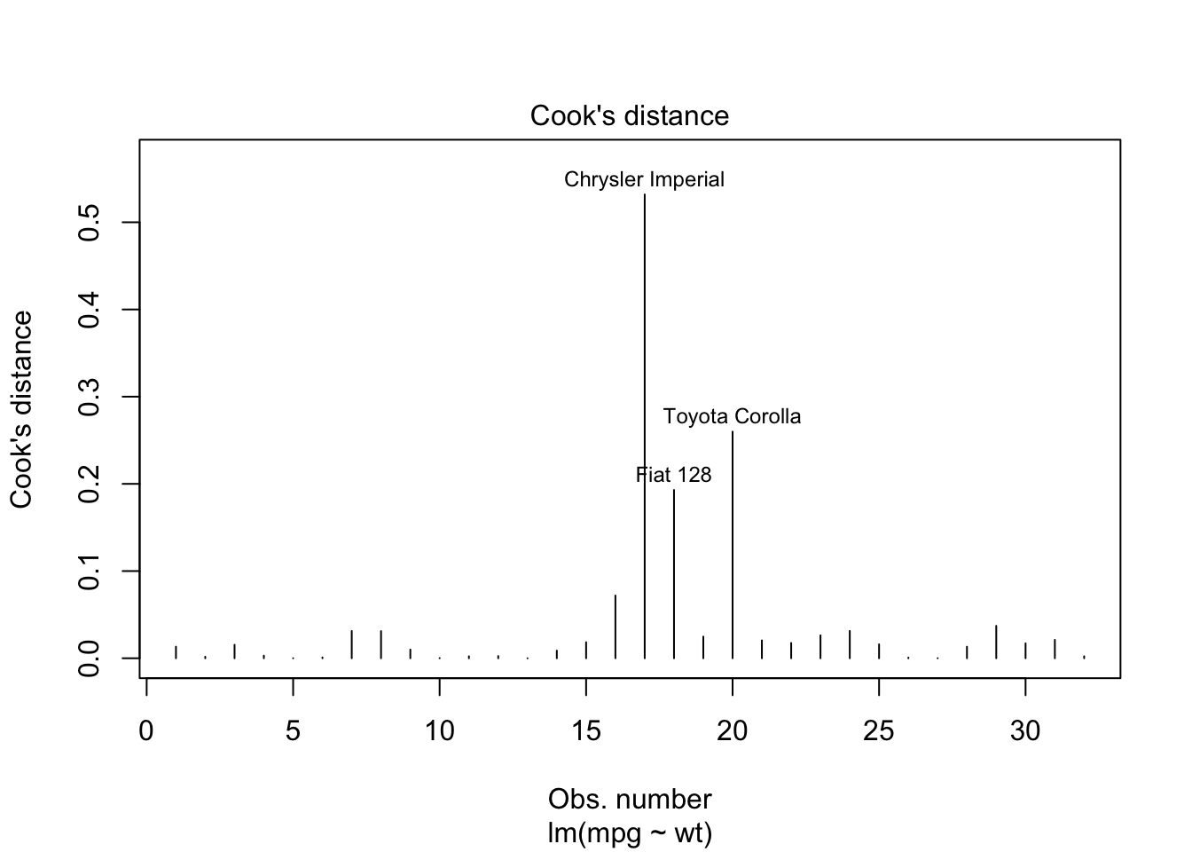
Once the model is fitted, it’s important to perform diagnostic checks to validate the model and ensure that the assumptions of linear regression have not been violated. This involves plotting the residuals to check for patterns that might suggest issues with linearity, independence, or homoscedasticity. Additionally, you can assess the normality of residuals using histograms or Q-Q plots and identify any outliers or influential points using plots like Cook’s distance.

# Plot residuals to check for linearity and homoscedasticity
plot(model, which = 1)  # Residuals vs Fitted

# Create a Q-Q plot to assess normality of residuals
qqnorm(model$residuals)
qqline(model$residuals)

# Identify potential outliers or influential points
plot(model, which = 4)  # Cook's distance

Explanation of the code:
- plot(model, which = 1): This command generates a residuals vs. fitted values plot to check for violations of linearity and homoscedasticity. A random scatter of residuals around the horizontal axis indicates that these assumptions are likely met. - qqnorm(model$residuals) and qqline(model$residuals): These functions create a Q-Q plot to assess whether the residuals are normally distributed. If the residuals follow a straight line, it suggests normality. - plot(model, which = 4): This generates a plot of Cook’s distance to identify potential outliers or influential points that might disproportionately affect the model’s results.

5.5.5 Step 5: Interpretation of Results

Interpreting the results involves understanding the significance of the model’s coefficients and evaluating the overall fit of the model.

# Extract the coefficients from the model
coefficients <- coef(summary(model))
print(coefficients)

             Estimate Std. Error   t value     Pr(>|t|)
(Intercept) 37.285126   1.877627 19.857575 8.241799e-19
wt          -5.344472   0.559101 -9.559044 1.293959e-10

# Calculate the confidence intervals for the coefficients
confint(model)

                2.5 %    97.5 %
(Intercept) 33.450500 41.119753
wt          -6.486308 -4.202635

# Evaluate the goodness-of-fit of the model
r_squared <- summary(model)$r.squared
adj_r_squared <- summary(model)$adj.r.squared
cat("R-squared:", r_squared, "\n")

R-squared: 0.7528328

cat("Adjusted R-squared:", adj_r_squared, "\n")

Adjusted R-squared: 0.7445939

Explanation of the code:
- coef(summary(model)): This function extracts the coefficients, standard errors, t-values, and p-values from the model summary, helping you assess the significance of the predictors. - confint(model): This function calculates confidence intervals for the model’s coefficients, providing a range within which the true coefficient values are likely to fall. - summary(model)$r.squared and summary(model)$adj.r.squared: These commands extract the R-squared and Adjusted R-squared values, which measure how well the model explains the variance in the dependent variable.

5.5.6 Step 6: Model Refinement and Reporting

After interpreting the initial results, you may refine the model by adding or removing variables to improve its performance. Finally, the findings should be summarized clearly, including the estimated coefficients, their significance, and the overall fit of the model.

# Example of refining the model by adding another predictor
model_refined <- lm(mpg ~ wt + hp, data = mtcars)
summary(model_refined)


Call:
lm(formula = mpg ~ wt + hp, data = mtcars)

Residuals:
   Min     1Q Median     3Q    Max 
-3.941 -1.600 -0.182  1.050  5.854 

Coefficients:
            Estimate Std. Error t value Pr(>|t|)    
(Intercept) 37.22727    1.59879  23.285  < 2e-16 ***
wt          -3.87783    0.63273  -6.129 1.12e-06 ***
hp          -0.03177    0.00903  -3.519  0.00145 ** 
---
Signif. codes:  0 '***' 0.001 '**' 0.01 '*' 0.05 '.' 0.1 ' ' 1

Residual standard error: 2.593 on 29 degrees of freedom
Multiple R-squared:  0.8268,    Adjusted R-squared:  0.8148 
F-statistic: 69.21 on 2 and 29 DF,  p-value: 9.109e-12

Explanation of the code:
- lm(mpg ~ wt + hp, data = mtcars): This function fits a refined linear regression model with two predictors (wt and hp). The summary of this model can help you determine whether the additional predictor improves the model’s performance.

5.6 Assessing the Goodness of Fit and Model Selection

After fitting a linear regression model, the next critical step is to evaluate how well the model captures the underlying relationships in the data and to determine whether the model is the best choice among potential alternatives. This evaluation is essential to ensure that the model not only fits the current data well but also generalizes effectively to new data. In this section, we will explore several key metrics and techniques used to assess the goodness of fit and guide model selection, helping to strike the right balance between model complexity and explanatory power.

$R^2$ as a Measure of Goodness of Fit

$R^2$, also known as the coefficient of determination, is a key metric used to evaluate how well a regression model fits the data. Specifically, $R^2$ indicates the proportion of the variance in the dependent variable that is predictable from the independent variables. It ranges from 0 to 1, where higher values suggest a better fit of the model to the data. For example, an $R^2$ value of 0.75 implies that 75% of the variability in the dependent variable is explained by the model, leaving 25% unexplained.

However, while $R^2$ provides useful information about the goodness of fit, it also has limitations. One significant limitation is that $R^2$ always increases as more predictors are added to the model, regardless of whether those predictors are truly significant. This can lead to overfitting, where the model fits the training data exceptionally well but may perform poorly on new, unseen data because it has captured noise rather than the underlying relationship.

Adjusted $R^2$ as a Model Selection Criterion

To address the limitations of $R^2$, adjusted $R^2$ is often used as a more reliable criterion for model selection. Adjusted $R^2$ modifies the $R^2$ value to account for the number of predictors in the model, thus penalizing the inclusion of unnecessary variables. The formula for adjusted $R^2$ is:

\[ \text{Adjusted } R^2 = 1 - \left( \frac{(1 - R^2)(n - 1)}{n - k - 1} \right) \]

where $n$ is the number of observations, and $k$ is the number of predictors. This adjustment ensures that adding a predictor to the model will only increase the adjusted $R^2$ if the predictor actually improves the model’s explanatory power.

Adjusted $R^2$ is particularly valuable when comparing models with different numbers of predictors. It helps determine whether the inclusion of additional variables genuinely enhances the model or if it merely adds unnecessary complexity. For instance, if adjusted $R^2$ increases when a new variable is added, this suggests that the variable contributes to a better explanation of the dependent variable. Conversely, if adjusted $R^2$ decreases, the added variable may be superfluous, indicating potential over fitting.

Unlike $R^2$, which only measures goodness of fit, adjusted $R^2$ serves as both a measure of goodness of fit and a model selection criterion. It balances the trade-off between fitting the data well and keeping the model as simple as possible. This makes adjusted $R^2$ a preferred metric for selecting the most parsimonious model that still explains the data effectively.

Residual Analysis for Goodness of Fit

Beyond $R^2$ and adjusted $R^2$, residual analysis is another crucial method for assessing the goodness of fit. Residuals, the differences between observed and predicted values, can reveal patterns that indicate potential issues with the model. Ideally, residuals should be randomly distributed without any systematic patterns. If residuals show a pattern, such as a trend or a funnel shape, it may suggest problems like non-linearity, heteroscedasticity (changing variance), or omitted variables.

By analyzing residuals, you can detect whether the model adequately captures the relationship between the independent and dependent variables. Residual plots, Q-Q plots, and histograms of residuals are commonly used tools for this purpose. Identifying issues early through residual analysis allows for model adjustments before finalizing the model.

Diagnosing and Addressing Model Issues

Even with careful model selection and goodness-of-fit assessment, issues such as multicollinearity, heteroscedasticity, and outliers may still arise.

Multicollinearity occurs when two or more predictors in the model are highly correlated, making it difficult to isolate the effect of each predictor. This can be diagnosed using Variance Inflation Factor (VIF) scores, where a VIF above 10 indicates significant multicollinearity. To address this, you can remove or combine highly correlated variables.
Heteroscedasticity refers to the situation where the variance of residuals is not constant across all levels of the independent variables. This violates one of the assumptions of linear regression and can lead to inefficient estimates. It can be detected using residual plots and addressed by transforming the dependent variable or using robust standard errors.
Outliers are data points that deviate significantly from the trend of the rest of the data. They can have a disproportionate impact on the model, skewing the results. Outliers can be identified through residual plots or influence plots like Cook’s distance. Depending on the context, outliers may be removed, or the model may be adjusted to reduce their influence.

5.7 Visualizing Regression Results Using R

After fitting a regression model and assessing its goodness of fit, the next crucial step is to visualize the results. Visualization not only helps in understanding the model’s behavior but also plays a key role in communicating the findings effectively. Through visualizations, you can easily identify trends, assess the relationship between variables, and convey the strength and significance of your model to others. In this section, we will explore how to plot the regression line using R, as well as how to enhance these visualizations with confidence intervals and annotations for a more comprehensive analysis.

Plotting the Regression Line

One of the simplest and most effective ways to visualize the results of a linear regression is to plot the data points and overlay the fitted regression line. This approach allows you to see how well the model captures the relationship between the independent and dependent variables.

# Fit the linear regression model
model <- lm(mpg ~ wt, data = mtcars)

# Create a scatter plot of the data
plot(mtcars$wt, mtcars$mpg, 
     main = "Scatter Plot with Regression Line",
     xlab = "Weight (1000 lbs)", 
     ylab = "Miles Per Gallon")

# Add the fitted regression line to the plot
abline(model, col = "blue", lwd = 2)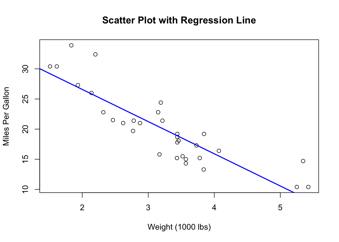

Explanation of the code:
- lm(mpg ~ wt, data = mtcars): This line fits a linear regression model where mpg is the dependent variable and wt (weight of the car) is the independent variable. - plot(mtcars$wt, mtcars$mpg): This command creates a scatter plot of the car weight (wt) against miles per gallon (mpg). The main argument adds a title to the plot, while xlab and ylab label the x and y axes, respectively. - abline(model, col = "blue", lwd = 2): This function adds the fitted regression line to the scatter plot. The col argument sets the color of the line to blue, and lwd (line width) increases the thickness of the line for better visibility.

By visualizing the regression line and enhancing it with confidence intervals and annotations, you can create a more informative and visually appealing representation of your regression model. These visualizations not only help in interpreting the results but also in effectively communicating the findings to others. With R’s powerful plotting capabilities, you can create clear and compelling graphics that highlight the key aspects of your regression analysis.

5.8 Summary of Key Concepts in Linear Regression Analysis

Introduction to Regression Analysis:
- Regression analysis is a statistical method used to examine relationships between variables.
- It is commonly applied in business contexts to make predictions, identify trends, and optimize processes.
- Linear regression models the relationship between a dependent variable and one or more independent variables.
What Is a Linear Regression Model?:
- The basic equation of a linear regression model is $Y = \beta_0 + \beta_1X + \epsilon$.
- $Y$: Dependent variable (outcome).
- $X$: Independent variable (predictor).
- $\beta_0$: Intercept, representing the expected value of $Y$ when $X = 0$.
- $\beta_1$: Slope, indicating the change in $Y$ for a one-unit change in $X$.
- $\epsilon$: Residual term, capturing the difference between observed and predicted values.
Assumptions of Simple Linear Regression:
- Linearity: The relationship between independent and dependent variables must be linear.
- Independence of Errors: Residuals should be independent of each other.
- Homoscedasticity: Residual variance should be constant across all levels of the independent variable.
- Normality of Residuals: Residuals should follow a normal distribution.
- Exogeneity: Independent variables should not be correlated with the error term.
- No Perfect Multicollinearity: Independent variables should not be perfectly correlated.
- No Specification Bias: The model must be correctly specified, including all relevant variables.
Interpreting Regression Output:
- Slope and Intercept: The slope quantifies the impact of $X$ on $Y$, and the intercept represents the baseline level of $Y$ when $X = 0$.
- Regression Model Summary: The summary provides estimates of coefficients, standard errors, t-values, p-values, R-squared, and more.
- Confidence Intervals: These provide a range within which the true coefficient values are likely to fall.
- Hypothesis Testing: The t-test and p-values determine the statistical significance of the regression coefficients.
Conducting a Linear Regression in R: Workflow Overview:
- Data Preparation: Load data and handle missing values.
- Exploratory Data Analysis (EDA): Use scatter plots and summary statistics to explore relationships.
- Model Fitting: Fit the model using the lm() function in R.
- Diagnostic Checks: Validate the model with residual plots, Q-Q plots, and Cook’s distance.
- Interpretation of Results: Analyze coefficients, confidence intervals, and goodness-of-fit metrics.
- Model Refinement and Reporting: Refine the model by adding or removing predictors and summarize findings.
Assessing the Goodness of Fit and Model Selection:
- $R^2$: Indicates the proportion of variance in $Y$ explained by $X$; higher values suggest a better fit.
- Adjusted $R^2$: Adjusts $R^2$ for the number of predictors, helping to prevent overfitting.
- Residual Analysis: Checks for patterns in residuals to identify potential issues with the model.
- Diagnosing Model Issues: Address multicollinearity, heteroscedasticity, and outliers.
Visualizing Regression Results Using R:
- Plotting the Regression Line: Use scatter plots with fitted regression lines to visualize the relationship between variables.
- Enhancements: Add confidence intervals and annotations to make the plot more informative.

5.9 Glossary of Terms

Adjusted $R^2$: A modified version of $R^2$ that adjusts for the number of predictors in the model, helping to prevent overfitting by penalizing the addition of unnecessary variables.
Coefficient: A number that represents the strength and direction of the relationship between a predictor (independent variable) and the outcome (dependent variable) in a regression model. In the equation $Y = \beta_0 + \beta_1X + \epsilon$, $\beta_0$ is the intercept, and $\beta_1$ is the slope.
Confidence Interval: A range of values, derived from the data, within which the true value of a regression coefficient is likely to fall, given a specified level of confidence (typically 95%).
Dependent Variable (Y): The outcome variable that the regression model aims to predict or explain based on the independent variable(s).
Exogeneity: The assumption that the independent variables are not correlated with the error term in a regression model. Violation of this assumption leads to biased and inconsistent estimates.
Heteroscedasticity: A condition in which the variance of the residuals (errors) is not constant across all levels of the independent variable. This violates the assumption of homoscedasticity and can lead to inefficient estimates.
Homoscedasticity: The assumption that the variance of residuals (errors) is constant across all levels of the independent variable in a regression model.
Independence of Errors: The assumption that the residuals (errors) in a regression model are independent of each other, meaning that the error of one observation does not influence the error of another.
Intercept ($\beta_0$): The expected value of the dependent variable ($Y$) when all the independent variables ($X$) are zero. It represents the baseline level of $Y$ in the regression equation.
Multicollinearity: A condition in multiple regression models where two or more independent variables are highly correlated, making it difficult to isolate the effect of each predictor on the dependent variable.
Multiple R-squared ($R^2$): A statistical measure that represents the proportion of variance in the dependent variable that is explained by the independent variable(s) in the model. It ranges from 0 to 1, with higher values indicating a better fit.
Normality of Residuals: The assumption that the residuals (errors) in a regression model are normally distributed. This assumption is important for making valid statistical inferences about the model’s coefficients.
Overfitting: A modeling error that occurs when a regression model is too complex, capturing noise in the data rather than the underlying relationship. This results in a model that performs well on the training data but poorly on new data.
Residual (Error): The difference between the observed value of the dependent variable and the value predicted by the regression model. Residuals are used to assess the fit of the model.
Residual Standard Error (RSE): A measure of the standard deviation of the residuals in a regression model. It reflects the average distance that the observed values fall from the regression line.
Slope ($\beta_1$): The coefficient that represents the change in the dependent variable ($Y$) for a one-unit change in the independent variable ($X$). It indicates the strength and direction of the relationship between $X$ and $Y$.
Specification Bias: A form of bias that occurs when a regression model is misspecified, either by omitting relevant variables or by including irrelevant ones. This can lead to incorrect estimates of the regression coefficients.
t-Value: A statistic that measures the number of standard deviations a coefficient estimate is from zero. It is used in hypothesis testing to determine whether a coefficient is significantly different from zero.
Variance Inflation Factor (VIF): A measure used to detect multicollinearity in a regression model. A high VIF indicates that an independent variable is highly correlated with other variables in the model, potentially leading to multicollinearity.