Curvature is common in business relationships: marketing spend shows diminishing returns, prices scale sublinearly with size, and operational outcomes vary nonlinearly over the day. This chapter shows how to model such patterns primarily with ordinary least squares (OLS) using transformations, low-order polynomials, and piecewise linear specifications. Advanced methods are briefly surveyed at the end.
Chapter Goals
Upon concluding this chapter, readers will be equipped with the skills to:
Diagnose non-linear patterns using exploratory graphics (e.g., smoothers, binned scatterplots) and residual structure from baseline linear models.
Select and justify functional forms—linear–log, log–linear, log–log, low-order polynomials, and piecewise (hinge) models—based on managerial meaning and data support.
Estimate OLS models with transformations, polynomial terms, and simple hinges; compute and interpret derivatives, semi-elasticities, and elasticities in business terms.
Locate and interpret turning points and slope changes, and translate these features into actionable managerial insights.
Validate specifications with residual diagnostics and light cross-validation, while guarding against overfitting and extrapolation beyond observed ranges.
Communicate non-linear effects clearly using prediction curves with confidence bands, and report impacts in meaningful units or percentages for decision-makers.
Recognize when OLS-based forms are insufficient and articulate when a brief, conceptual comparison to advanced methods (e.g., GAMs, tree-based models) is warranted, without delving into implementation.
Datasets referenced in this chapter (open access)
Ames Housing (real estate pricing). Source: De Cock (2011), JSE; available via the AmesHousing package
Diamonds (retail pricing). Source: ggplot2::diamonds
Inside Airbnb (hospitality pricing). Source: insideairbnb.com
Advertising (marketing mix). Source: ISLR website (Advertising.csv)
Wage (compensation analytics). Source: ISLR2::Wage
mpg (automotive fuel economy). Source: ggplot2::mpg
Bike Sharing (demand vs temperature). Source: UCI Machine Learning Repository
NYC Taxi trips (transport pricing; sample recommended) and NYC TLC rate card
USPS Notice 123 (tiered shipping)
nycflights13 (operations; delays by hour). Source: nycflights13 package (CC0)
Solar PV learning curve (experience effects). Source: Our World in Data
AmesHousing: use AmesHousing::make_ames()
Diamonds/mpg: available in ggplot2 as ggplot2::diamonds ggplot2::mpg
Advertising.csv: download from the ISLR site, then read with readr::read_csv("Advertising.csv")
Wage: available as ISLR2::Wage
Inside Airbnb: choose a city/date and download listings.csv.gz from the data portal
UCI Bike Sharing: download day.csv and hour.csv from the repository
NYC TLC trips: sample a manageable subset of monthly CSVs; pair with the official fare schedule
USPS Notice 123: build a compact weight–price table from the online price list
nycflights13: nycflights13::flights
Our World in Data solar: download PV price and capacity series and join into a tidy table
Motivation: seeing non-linearity early
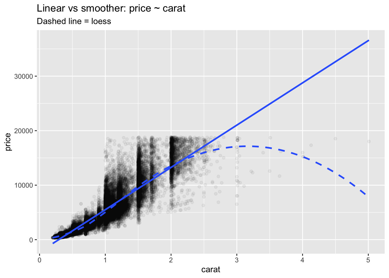
Anscombe’s reminder: identical summaries can mask very different shapes. Always visualize.
# Visual comparison of linear fit vs flexible smoother (power-law context) ggplot (diamonds, aes (carat, price)) + geom_point (alpha = 0.05 ) + geom_smooth (method = "lm" , se = FALSE ) + geom_smooth (method = "loess" , se = FALSE , linetype = "dashed" ) + labs (title = "Linear vs smoother: price ~ carat" , subtitle = "Dashed line = loess" )
`geom_smooth()` using formula = 'y ~ x'
`geom_smooth()` using formula = 'y ~ x'
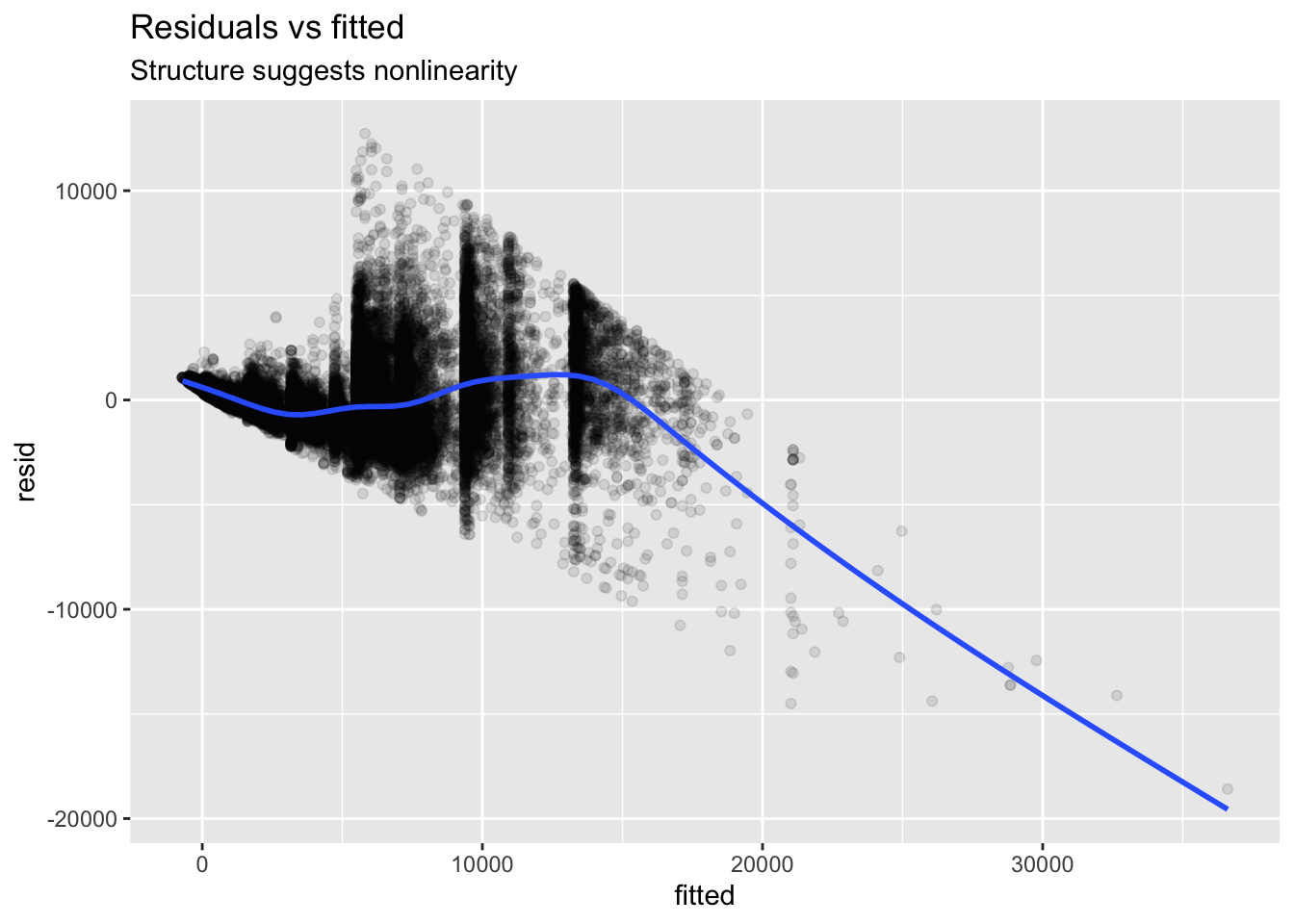
Residual patterns often reveal missed curvature.
<- lm (price ~ carat, data = diamonds)<- tibble (fitted = fitted (m_lin),resid = resid (m_lin)ggplot (aug, aes (fitted, resid)) + geom_point (alpha = 0.1 ) + geom_smooth (se = FALSE ) + labs (title = "Residuals vs fitted" , subtitle = "Structure suggests nonlinearity" )
`geom_smooth()` using method = 'gam' and formula = 'y ~ s(x, bs = "cs")'
Modeling non-linearity with OLS (concepts)
Transformations: linear, linear–log, log–linear, log–log
Low-order polynomials: quadratic, cubic; center/scale to reduce collinearity
Piecewise linear (hinge): add \(\max(0, X-k)\) for a knot \(k\) ; justify with business logic or policy thresholds
Examples and mini-applications
Constant-elasticity pricing (log–log)
Diamonds (retail pricing): price vs carat
Source: ggplot2::diamonds
<- lm (log (price) ~ log (carat), data = diamonds)summary (m_loglog_diamonds) # elasticity = coef on log(carat)
Call:
lm(formula = log(price) ~ log(carat), data = diamonds)

Residuals:
     Min       1Q   Median       3Q      Max
-1.50833 -0.16951 -0.00591  0.16637  1.33793

Coefficients:
            Estimate Std. Error t value Pr(>|t|)
(Intercept) 8.448661   0.001365  6190.9   <2e-16 ***
log(carat)  1.675817   0.001934   866.6   <2e-16 ***
---
Signif. codes:  0 '***' 0.001 '**' 0.01 '*' 0.05 '.' 0.1 ' ' 1

Residual standard error: 0.2627 on 53938 degrees of freedom
Multiple R-squared:  0.933, Adjusted R-squared:  0.933
F-statistic: 7.51e+05 on 1 and 53938 DF,  p-value: < 2.2e-16
Ames Housing (real estate pricing): sale price vs living area
Source: De Cock (2011), JSE; available via the AmesHousing package
<- AmesHousing:: make_ames ()<- lm (log (Sale_Price) ~ log (Gr_Liv_Area), data = ames)summary (m_loglog_ames)
Call:
lm(formula = log(Sale_Price) ~ log(Gr_Liv_Area), data = ames)

Residuals:
    Min      1Q  Median      3Q     Max
-2.0778 -0.1465  0.0264  0.1740  0.8602

Coefficients:
                 Estimate Std. Error t value Pr(>|t|)
(Intercept)       5.43019    0.11644   46.63   <2e-16 ***
log(Gr_Liv_Area)  0.90781    0.01602   56.66   <2e-16 ***
---
Signif. codes:  0 '***' 0.001 '**' 0.01 '*' 0.05 '.' 0.1 ' ' 1

Residual standard error: 0.2816 on 2928 degrees of freedom
Multiple R-squared:  0.523, Adjusted R-squared:  0.5228
F-statistic:  3210 on 1 and 2928 DF,  p-value: < 2.2e-16
Diminishing returns to spend (linear–log)
ISLR Advertising: Sales ~ log(TV) (extend to other channels as needed)
Source: ISLR website (Advertising.csv)
<- read_csv ("https://www.statlearning.com/s/Advertising.csv" , show_col_types = FALSE )
New names:
• `` -> `...1`
<- lm (sales ~ log (TV), data = adv)summary (m_linlog_adv)
Call:
lm(formula = sales ~ log(TV), data = adv)

Residuals:
    Min      1Q  Median      3Q     Max
-5.9318 -2.6777 -0.2758  2.1227  9.2654

Coefficients:
            Estimate Std. Error t value Pr(>|t|)
(Intercept)  -4.2026     1.1623  -3.616  0.00038 ***
log(TV)       3.9009     0.2432  16.038  < 2e-16 ***
---
Signif. codes:  0 '***' 0.001 '**' 0.01 '*' 0.05 '.' 0.1 ' ' 1

Residual standard error: 3.45 on 198 degrees of freedom
Multiple R-squared:  0.565, Adjusted R-squared:  0.5628
F-statistic: 257.2 on 1 and 198 DF,  p-value: < 2.2e-16
Semi-elasticities in compensation (log–linear)
ISLR Wage: log(wage) ~ age + age² (optionally add tenure, education)
data (Wage, package = "ISLR2" )<- lm (log (wage) ~ age + I (age^ 2 ), data = Wage)summary (m_loglin_wage)
Call:
lm(formula = log(wage) ~ age + I(age^2), data = Wage)

Residuals:
     Min       1Q   Median       3Q      Max
-1.72742 -0.19431  0.00655  0.18995  1.13251

Coefficients:
              Estimate Std. Error t value Pr(>|t|)
(Intercept)  3.468e+00  6.810e-02   50.93   <2e-16 ***
age          5.166e-02  3.232e-03   15.98   <2e-16 ***
I(age^2)    -5.202e-04  3.685e-05  -14.12   <2e-16 ***
---
Signif. codes:  0 '***' 0.001 '**' 0.01 '*' 0.05 '.' 0.1 ' ' 1

Residual standard error: 0.3325 on 2997 degrees of freedom
Multiple R-squared:  0.1069,    Adjusted R-squared:  0.1063
F-statistic: 179.3 on 2 and 2997 DF,  p-value: < 2.2e-16
Quadratic curvature and turning points
Automotive fuel economy: hwy ~ displ + displ²
<- lm (hwy ~ displ + I (displ^ 2 ), data = mpg)<- - coef (m_quad_mpg)["displ" ] / (2 * coef (m_quad_mpg)["I(displ^2)" ])
Bike demand vs temperature (UCI Bike Sharing): cnt ~ temp + temp²day.csv from the UCI repository and place at data/bike_day.csv
Source: UCI Machine Learning Repository (Bike Sharing Dataset)
# bike_day <- read_csv("data/bike_day.csv")
# m_quad_bike <- lm(cnt ~ temp + I(temp^2), data = bike_day)
# summary(m_quad_bike)
Piecewise (hinge) models from pricing rules
NYC Taxi: total fare vs distance with base fee and per-mile segments. Use a sampled trips file (e.g., data/nyc_taxi_sample.csv) and the official rate card to justify the knot(s)
Source: NYC Taxi & Limousine Commission trip records; NYC TLC rate card
# taxi <- read_csv("data/nyc_taxi_sample.csv")
# taxi <- taxi %>% mutate(after1 = pmax(trip_distance - 1, 0))
# m_hinge_taxi <- lm(total_amount ~ trip_distance + after1, data = taxi)
# summary(m_hinge_taxi)
USPS shipping: postage vs weight shows step/tier pricing (use hinges at ounce thresholds)
# usps <- tribble(
#   ~weight_oz, ~price_usd,
#   1, 0.68,
#   2, 0.92,
#   3, 1.16,
#   3.5, 1.40
# )
# usps <- usps %>% mutate(after1 = pmax(weight_oz - 1, 0),
#                         after2 = pmax(weight_oz - 2, 0),
#                         after3 = pmax(weight_oz - 3, 0))
# m_hinge_usps <- lm(price_usd ~ weight_oz + after1 + after2 + after3, data = usps)
# summary(m_hinge_usps)
Smooth time-of-day curvature (splines for contrast)
Airline operations: departure delay vs hour (nycflights13). Splines provide a compact, smooth alternative to high-order polynomials
Source: nycflights13 package (CC0)
<- nycflights13:: flights %>% filter (! is.na (dep_delay), ! is.na (hour))<- lm (dep_delay ~ bs (hour, df = 4 ), data = fl)summary (m_spline_fl)
Call:
lm(formula = dep_delay ~ bs(hour, df = 4), data = fl)

Residuals:
    Min      1Q  Median      3Q     Max
 -66.09  -18.26   -9.49   -1.03 1296.23

Coefficients:
                  Estimate Std. Error t value Pr(>|t|)
(Intercept)         0.3436     0.4035   0.852    0.394
bs(hour, df = 4)1   3.2272     0.7622   4.234  2.3e-05 ***
bs(hour, df = 4)2   7.0820     0.5462  12.966  < 2e-16 ***
bs(hour, df = 4)3  32.5465     0.7685  42.349  < 2e-16 ***
bs(hour, df = 4)4  16.3872     0.6992  23.436  < 2e-16 ***
---
Signif. codes:  0 '***' 0.001 '**' 0.01 '*' 0.05 '.' 0.1 ' ' 1

Residual standard error: 39.38 on 328516 degrees of freedom
Multiple R-squared:  0.04081,   Adjusted R-squared:  0.0408
F-statistic:  3494 on 4 and 328516 DF,  p-value: < 2.2e-16
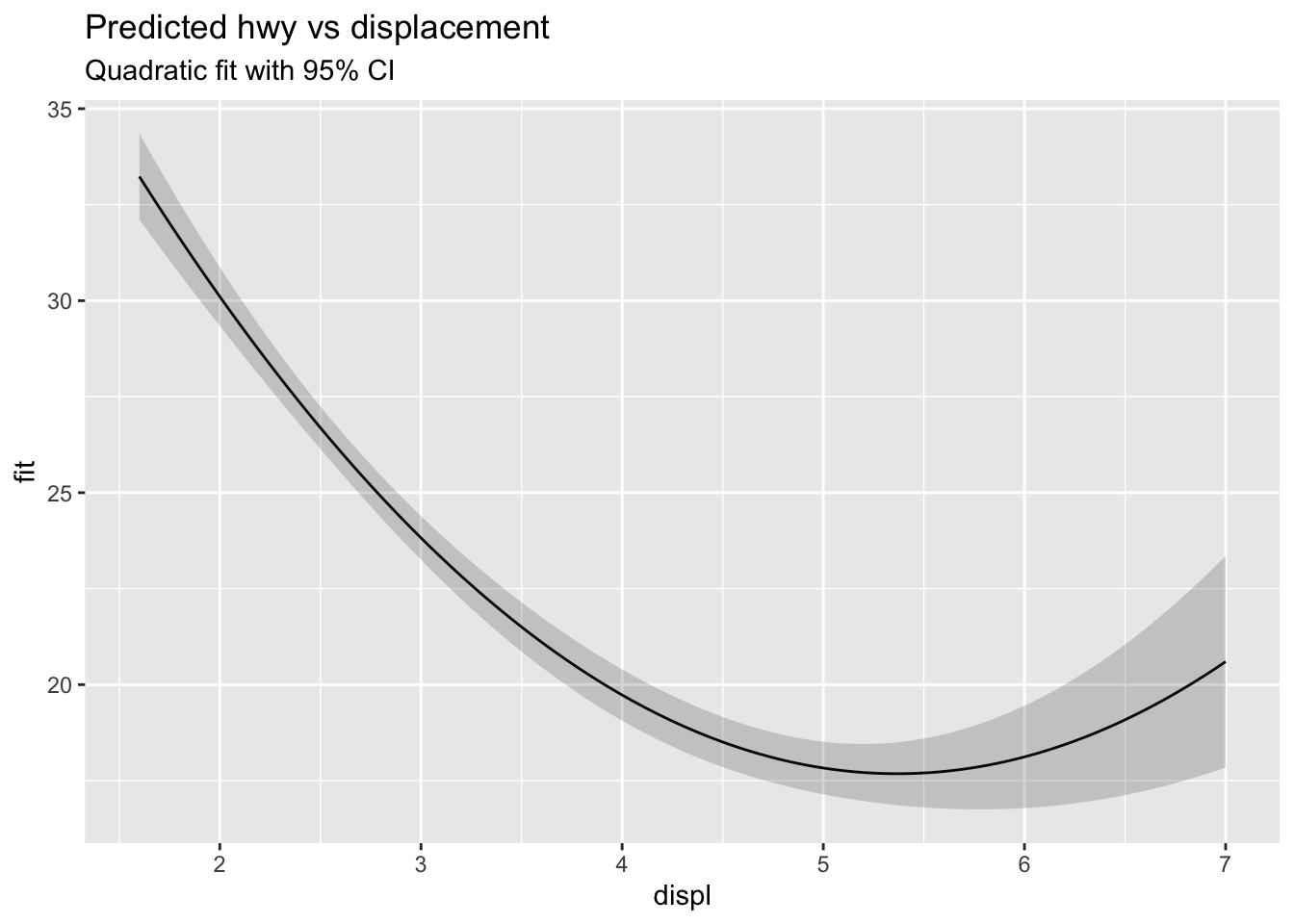
Visualize effect curve with confidence band for any fitted model
<- tibble (displ = seq (min (mpg$ displ), max (mpg$ displ), length.out = 200 ))<- cbind (newx, predict (m_quad_mpg, newdata = newx, interval = "confidence" ))ggplot (preds, aes (displ, fit)) + geom_line () + geom_ribbon (aes (ymin = lwr, ymax = upr), alpha = 0.2 ) + labs (title = "Predicted hwy vs displacement" , subtitle = "Quadratic fit with 95% CI" )
Learning curves and experience effects
Solar PV learning curve: log(price_per_watt) ~ log(cumulative_capacity)solar_df with columns price_watt, cum_capacity
Source: Our World in Data
# solar_df <- read_csv("data/owid_solar_joined.csv")
# m_lc <- lm(log(price_watt) ~ log(cum_capacity), data = solar_df)
# lr <- 1 - 2^(coef(m_lc)[2])   # learning rate per doubling of capacity
# lr
Diagnostics and validation
Recheck residuals after transformation; look for remaining curvature and heteroscedasticity
Compare forms with light cross-validation (e.g., repeated splits or K-fold)
Avoid high-order oscillations; do not extrapolate beyond observed \(X\)
set.seed (123 )<- sample.int (nrow (mpg), size = floor (0.8 * nrow (mpg)))<- mpg[idx, ]; m_test <- mpg[- idx, ]<- lm (hwy ~ displ, data = m_train)<- lm (hwy ~ displ + I (displ^ 2 ), data = m_train)<- function (y, yhat) sqrt (mean ((y - yhat)^ 2 ))<- rmse (m_test$ hwy, predict (m_lin_mpg, newdata = m_test))<- rmse (m_test$ hwy, predict (m_quad_mpg, newdata = m_test))tibble (model = c ("linear" ,"quadratic" ), rmse = c (rmse_lin, rmse_quad))
Communicating effects to managers
Translate derivatives into plain language: where gains diminish, where risks rise
Report elasticities or semi-elasticities at meaningful \(X\) values
Plot predicted curves within supported ranges; mark turning points and slope changes
For pricing and demand, log–log elasticities communicate clearly. For costs, linear or linear–log forms often align with managerial expectations
Advanced methods (brief survey; implementations beyond scope)
Generalized Additive Models (GAM): smooth, additive curves with interpretable partial effects
Tree-based ensembles (random forests, gradient boosting): flexible prediction with interactions and nonlinearity
Local methods (k-nearest neighbors): simple non-parametric baseline
Implementation of these advanced methods is beyond the scope of this chapter; use them as benchmarks when OLS forms clearly underfit
Summary of Key Concepts
Curvature is common in business data; start by visualizing on the original scale
Choose the simplest form that removes residual structure and communicates clearly
Transformations provide interpretable parameters: linear–log for diminishing returns, log–linear for percent impacts, log–log for elasticities
Low-order polynomials capture smooth curvature; compute turning points at \(X^{\star} =-\beta_1/(2\beta_2)\) when applicable
Piecewise linear models align with policy thresholds and pricing tiers; justify knot placement with business logic
Validate with residual checks and light cross-validation; avoid extrapolation beyond observed \(X\)
Communicate effects using prediction curves with confidence bands and translate into percent or unit impacts for decision-makers
Glossary of Terms
Elasticity: the percent change in \(Y\) associated with a 1% change in \(X\) ; in log–log models, equals the slope coefficient
Semi-elasticity: the percent change in \(Y\) per unit change in \(X\) (log–linear) or the unit change in \(Y\) per 1% change in \(X\) (linear–log)
Turning point: the \(X\) value where a quadratic’s marginal effect \(dY/dX=\beta_1+2\beta_2 X\) equals zero, \(X^{\star} =-\beta_1/(2\beta_2)\)
Hinge term: a piecewise linear basis function \(\max(0, X-k)\) that allows a slope change at knot \(k\)
Knot: the value of \(X\) where the slope is permitted to change in a piecewise model
Partial residual plot: a visualization of a predictor’s adjusted relationship with the outcome after accounting for other covariates
Smoother: a flexible curve (e.g., loess) used in EDA to reveal non-linear patterns without specifying a parametric form
Overfitting: modeling noise as if it were signal; often manifests with high-order polynomials or excessive flexibility
Extrapolation: using the model to predict beyond the observed range of \(X\) , where functional-form assumptions are least reliable