In this case study, we examine whether it is commercially advantageous for automakers to adopt a new fuel efficiency technology that increases miles per gallon (MPG) by 10 but also raises production costs by $1,000 per vehicle. As the automotive industry faces growing demand for eco-friendly vehicles and stricter environmental regulations, manufacturers are under pressure to improve fuel efficiency while maintaining profitability. This study aims to assess whether the increased production costs can be justified by a corresponding increase in the Manufacturer’s Suggested Retail Price (MSRP), and whether consumers are willing to pay more for vehicles that offer better fuel efficiency.
The adoption of fuel-efficient technologies, such as hybrid systems and electric powertrains, has become a key focus for automakers seeking to remain competitive in an evolving market. However, the question remains: will consumers be willing to pay a higher price for these advancements? This case study will explore how improvements in fuel efficiency affect vehicle pricing, customer demand, and overall business outcomes.
We will use real-world data on various car models, brands, and their features to analyze the relationship between fuel efficiency and MSRP. The goal is to determine if the cost increase associated with the new technology can be offset by raising prices without negatively impacting demand. By examining the financial trade-offs involved, this study will provide insights into whether adopting fuel-efficient technologies is a sound business strategy for automakers.
8.2 Research Question and Decision Criteria
The primary objective of this case study is to determine whether automakers should adopt a new fuel efficiency technology that increases miles per gallon (MPG) by 10 but also adds $1,000 to the production cost of each vehicle. The central research question revolves around whether the increased production cost can be compensated by a higher Manufacturer’s Suggested Retail Price (MSRP), and whether consumers will be willing to pay a premium for improved fuel efficiency. Although a complete analysis requires addressing several important sub-questions, this chapter will focus specifically on the first question: Can the MSRP be increased enough to offset the $1,000 production cost?
To explore this question, we will model the relationship between MPG and MSRP to determine how much of a price increase can be justified by the additional 10 MPG. If the increase in MSRP is sufficient to cover or exceed the $1,000 cost without negatively affecting consumer demand, adopting the technology could be deemed a viable strategy. Additionally, while this chapter concentrates on pricing, other critical considerations must be explored to provide a more comprehensive answer to the research question.
Beyond pricing, it is essential to evaluate the impact of fuel efficiency on customer demand and preferences. Understanding whether an increase in MSRP due to higher fuel efficiency will lead to a drop in sales volume is a key factor in determining the technology’s success. Furthermore, long-term consumer value must be considered by comparing the projected fuel savings from the 10 MPG improvement over a typical ownership period (e.g., five years) against the higher MSRP. This will help determine whether consumers perceive sufficient savings to justify paying the premium.
Another factor to examine is how the technology affects a vehicle’s competitiveness in the market. The MSRP increase due to the new technology should not push the vehicle into a higher price segment where it may lose competitiveness against similarly priced models. Finally, from a business perspective, it is crucial to assess the sustainability of the $1,000 production cost increase. A financial analysis will help determine whether this cost increase can be offset by the higher MSRP without negatively impacting profit margins or long-term financial health.
While the focus of this chapter is on determining whether the MSRP can be raised enough to cover the additional production costs, addressing these other sub-questions will be necessary to make a fully informed decision about the viability of adopting the new fuel efficiency technology.
8.3 Data Overview
In this case study, we will be working with a simulated dataset that contains detailed information about various vehicles, their features, performance metrics, and market positioning. This dataset provides insights into important variables such as manufacturer, model, fuel efficiency, pricing, and customer ratings, which are critical to assessing the impact of adopting new fuel efficiency technology. The dataset used for this analysis can be accessed at the following link: https://ljkelly3141.github.io/real-world-statistics-with-r/data/car_price.xlsx.
Below is an overview of the relevant variables in the dataset that will be used in our analysis:
Brand: This categorical variable indicates the manufacturer of the vehicle, such as Tesla, Toyota, or Ford. It is a nominal variable, meaning there is no inherent ranking or order among the different brands.
Model: This variable specifies the particular model of the vehicle, such as Camry or Model 3. Like Brand, it is a nominal categorical variable with no ranking.
Trim: This nominal categorical variable describes the version or package level of the vehicle model, offering different features and specifications depending on the trim level.
Trim Level: Unlike the Trim variable, Trim Level is an ordinal categorical variable that indicates the luxury or feature set of the vehicle. It has an inherent order, ranging from Base to Medium and Premium.
Style: This categorical variable refers to the body type of the vehicle, such as Sedan, SUV, or Pickup. It is nominal, with no inherent ranking among styles.
Size: This ordinal categorical variable describes the size class of the vehicle, such as Compact, Midsize, or Full-size. The size categories follow a logical order based on vehicle dimensions.
MSRP (USD): This is a numeric variable representing the Manufacturer’s Suggested Retail Price, which is the base price of the vehicle in U.S. dollars.
Energy Efficiency (MPG): Measured in miles per gallon, this numeric variable provides a key indicator of the vehicle’s fuel efficiency, which is a central focus of this case study.
Horsepower: Another numeric variable, horsepower measures the power output of the vehicle’s engine, which influences both performance and fuel consumption.
Engine Size (L): This numeric variable indicates the engine displacement, measured in liters. Larger engines typically offer more power but may reduce fuel efficiency.
Customer Rating: A numeric variable representing the customer satisfaction rating on a scale of 1 to 5 stars. This provides insights into consumer preferences and their perceived value of the vehicle.
Safety Rating: This numeric variable reflects the vehicle’s safety performance, based on crash test results, with ratings between 1 and 5 stars.
Hybrid: A nominal categorical variable indicating whether the vehicle uses hybrid technology (Hybrid/Non-Hybrid).
Electric: This nominal categorical variable specifies whether the vehicle is fully electric (Electric/Non-Electric).
Four_Wheel_Drive: A nominal variable indicating whether the vehicle is equipped with four-wheel drive (4WD/2WD).
Sunroof: A nominal categorical variable that indicates whether the vehicle is equipped with a sunroof (Yes/No).
Bluetooth: Another nominal variable specifying whether the vehicle has Bluetooth connectivity (Yes/No).
Backup Camera: This nominal variable shows whether the vehicle includes a backup camera (Yes/No).
Main Market: A nominal categorical variable indicating the primary market where the vehicle is sold, either North America or Europe.
Average Annual Cost of Ownership (USD): This numeric variable estimates the total annual cost of owning the vehicle, including maintenance, insurance, fuel costs, and depreciation.
Below is a summary table of the variables:
Variable Name
Description
Data Type
Categorical Type
Brand
Manufacturer of the vehicle (e.g., Tesla, Toyota, Ford)
Categorical
Nominal
Model
Specific model of the vehicle (e.g., Camry, Model 3)
Categorical
Nominal
Trim
Version or package level of the vehicle model
Categorical
Nominal
Trim_Level
Luxury or feature set of the vehicle (Base, Medium, Premium)
Categorical
Ordinal
Style
Body type of the vehicle (Sedan, SUV, Pickup)
Categorical
Nominal
Size
Size class of the vehicle (Compact, Midsize, Full-size)
Categorical
Ordinal
MSRP (USD)
Manufacturer’s Suggested Retail Price in U.S. dollars
Numeric
-
Energy Efficiency (MPG)
Fuel efficiency measured in miles per gallon (MPG)
Numeric
-
Horsepower
Power output of the vehicle, measured in horsepower (HP)
Numeric
-
Engine Size (L)
Engine displacement measured in liters
Numeric
-
Customer Rating
Customer satisfaction rating (out of 5 stars)
Numeric
-
Safety Rating
Safety rating based on crash test performance (1-5 stars)
Numeric
-
Hybrid
Whether the vehicle is a hybrid (Hybrid/Non-Hybrid)
Categorical
Nominal
Electric
Whether the vehicle is fully electric (Electric/Non-Electric)
Categorical
Nominal
Four_Wheel_Drive
Indicates if the vehicle has 4WD (4WD/2WD)
Categorical
Nominal
Sunroof
Whether the vehicle has a sunroof (Yes/No)
Categorical
Nominal
Bluetooth
Whether the vehicle has Bluetooth connectivity (Yes/No)
Categorical
Nominal
Backup Camera
Whether the vehicle has a backup camera (Yes/No)
Categorical
Nominal
Main Market
The primary market where the vehicle is sold (North America/Europe)
Categorical
Nominal
Average Annual Cost of Ownership (USD)
Estimated total annual cost of owning the vehicle in USD
Numeric
-
This simulated dataset provides a comprehensive view of the vehicles’ key characteristics, which will be crucial for analyzing the impact of the new fuel efficiency technology on MSRP and other business outcomes. By exploring the relationships among these variables, we can better understand how consumers value fuel efficiency and whether an increase in MSRP is justified by improved fuel economy.
8.4 Loading and Preparing the Data
To begin the analysis, we first need to load the dataset containing information about various vehicle models, including key variables such as Manufacturer’s Suggested Retail Price (MSRP), Fuel Efficiency (MPG), and other features. The data is available in both CSV and Excel formats and can be loaded into R using the appropriate functions.
For this case study, the data has been made available in an Excel file, which can be accessed online. To ensure that the column names in the dataset are preserved in their original form (including spaces and special characters), we will use the openxlsx::read.xlsx() function with specific arguments that prevent automatic renaming of the columns. Here is how we load the data:
# Install the openxlsx package if not installedif (!require(openxlsx)) install.packages("openxlsx")
Loading required package: openxlsx
library(openxlsx)# Read the Excel file directly from the URLcar_price <-read.xlsx("https://ljkelly3141.github.io/real-world-statistics-with-r/data/car_price.xlsx",check.names =FALSE,sep.names =" ")# View the first few rows of the datasethead(car_price)
Brand
Model
Trim
Trim Level
Style
Size
MSRP (USD)
Energy Efficiency (MPG)
Horsepower
Engine Size (L)
Customer Rating
Safety Rating
Hybrid
Electric
Four_Wheel_Drive
Sunroof
Bluetooth
Backup_Camera
Main Market
Average Annual Cost of Ownership (USD)
Toyota
Camry
LE
Base
Sedan
Midsize
2.9e+04
32
203
2.5
4.5
5
Non-Hybrid
Non-Electric
2WD
Sunroof
Bluetooth
Backup Camera
North America
6.2e+03
Toyota
Camry
XSE
Medium
Sedan
Midsize
3.4e+04
31
301
3.5
4.7
5
Non-Hybrid
Non-Electric
2WD
Sunroof
Bluetooth
Backup Camera
North America
6.4e+03
Toyota
Camry
Hybrid
Premium
Sedan
Midsize
3.7e+04
50
208
2.5
4.8
5
Hybrid
2WD
Sunroof
Bluetooth
Backup Camera
North America
5.8e+03
Ford
F-150
XLT
Base
Pickup
Full-size
5.2e+04
20
290
3.3
4.4
5
Non-Hybrid
4WD
Bluetooth
Backup Camera
North America
9.1e+03
Ford
F-150
Lariat
Medium
Pickup
Full-size
6.1e+04
18
400
5
4.6
5
Non-Hybrid
4WD
Sunroof
Bluetooth
Backup Camera
North America
9.5e+03
Ford
F-150
Platinum
Premium
Pickup
Full-size
7.2e+04
18
400
5
4.8
5
Non-Hybrid
4WD
Sunroof
Bluetooth
Backup Camera
North America
9.8e+03
WarningHandling Variable Names in R: Preventing Automatic Changes
When importing datasets into R, some functions automatically modify variable names to ensure they follow R’s naming conventions. This can happen when column names contain spaces, special characters, or start with numbers, which may lead to unexpected changes in the names.
1. Why Variable Names Are Changed
Many import functions in R automatically adjust variable names to comply with older versions of R’s stricter naming rules: - Variable names must begin with a letter and can only contain letters, numbers, dots (.), or underscores (_). - Special characters like spaces, parentheses, and operators (e.g., +, -, *) are not allowed. - Names cannot start with numbers (e.g., 1st_variable is invalid).
These restrictions often result in automatic changes to column names, such as replacing spaces with dots or underscores. For example, a column named "MSRP (USD)" might become "MSRP.USD".
2. Preventing Name Changes in Different Import Functions
The read.csv() function in base R uses an argument called check.names. By default, it is set to TRUE, meaning that R will automatically adjust column names to valid R names. To prevent this, set check.names = FALSE.
# Prevent read.csv() from changing column namesdata <-read.csv("your_file.csv", check.names =FALSE)
The read_excel() function from the readxl package preserves original column names by default, so no additional argument is needed to prevent name changes.
# Read the Excel file while preserving the original column namesdata <-read_excel("your_file.xlsx")
By default, read.xlsx() from the openxlsx package modifies column names, replacing spaces with dots (.). To preserve the original column names, you need to use two arguments: - check.names = FALSE to avoid modifying the names. - sep.names = " " to specify that spaces should be preserved instead of being replaced by dots or underscores.
# Read the Excel file while preserving the original column names and spacesdata <-read.xlsx("your_file.xlsx", check.names =FALSE, sep.names =" ")
By using both check.names = FALSE and sep.names = " ", you can fully preserve the original names, including spaces and special characters, when importing data using openxlsx::read.xlsx().
3. Using Backticks for Non-Standard Variable Names in R
In R, backticks () are used to reference variable names that contain spaces, special characters, or start with numbers. Normally, variable names must follow strict rules (e.g., starting with a letter, no spaces), but backticks allow you to bypass these restrictions.
For example, if a dataset contains a column named "MSRP (USD)", you can reference it using backticks:
# Accessing a variable with spaces or special characters using backticksdata$`MSRP (USD)`
Backticks are essential when working with non-standard names that would otherwise cause errors in R code.
8.5 Exploratory Analysis
8.5.1 Summary Statistics for Numeric Variables
To better understand the distribution of the numeric variables in the dataset, we will compute summary statistics such as means and standard deviations. These metrics will provide insights into the central tendency and variability of key variables like MSRP (USD), Energy Efficiency (MPG), Horsepower, Engine Size (L), Customer Rating, Safety Rating, and Average Annual Cost of Ownership (USD).
# Load the psych packagelibrary("psych")# Compute summary statistics for numeric variablesdescribe(car_price, omit =TRUE, skew =FALSE, ranges =FALSE)
names
vars
n
mean
sd
se
MSRP (USD)
7
44
4.73e+04
1.54e+04
2.32e+03
Energy Efficiency (MPG)
8
44
33.2
22.1
3.33
Horsepower
9
44
259
84.8
12.8
Engine Size (L)
10
42
2.75
1.29
0.199
Customer Rating
11
44
4.63
0.121
0.0182
Safety Rating
12
44
4.73
0.544
0.082
Average Annual Cost of Ownership (USD)
20
44
7.3e+03
1.61e+03
243
This code uses the describe() function from the psych package to compute key summary statistics for the dataset, including means and standard deviations. The omit = TRUE argument ensures that missing values are excluded from the calculations, while skew = FALSE and ranges = FALSE simplify the output by excluding skewness and range information for now.
8.5.2 Identify Outliers
Next, we identify potential outliers in key numeric variables. Outliers are extreme values that fall outside the expected range and could influence the results of the analysis. While we will not filter or remove any data at this stage, it is important to flag these values for consideration during the modeling process.
To identify outliers, we use the interquartile range (IQR) method, which flags values that fall below the first quartile (Q1) minus 1.5 times the IQR or above the third quartile (Q3) plus 1.5 times the IQR. Below is the code for identifying outliers in MSRP (USD) and Energy Efficiency (MPG).
This code identifies outliers in the MSRP (USD) and Energy Efficiency (MPG) variables using the Tukey method. MPG_Outlier flags vehicles with extreme values in fuel efficiency (MPG). Here are the observations flaged as outliers:
# View the dataset with outliers flaggedcar_price[car_price$MPG_Outlier,]
Brand
Model
Trim
Trim Level
Style
Size
MSRP (USD)
Energy Efficiency (MPG)
Horsepower
Engine Size (L)
Customer Rating
Safety Rating
Hybrid
Electric
Four_Wheel_Drive
Sunroof
Bluetooth
Backup_Camera
Main Market
Average Annual Cost of Ownership (USD)
MPG_Outlier
Toyota
Camry
Hybrid
Premium
Sedan
Midsize
3.7e+04
50
208
2.5
4.8
5
Hybrid
2WD
Sunroof
Bluetooth
Backup Camera
North America
5.8e+03
TRUE
Tesla
Model 3
Standard Range Plus
Base
Sedan
Midsize
4.2e+04
125
258
4.8
5
Hybrid
Electric
2WD
Sunroof
Bluetooth
Backup Camera
North America
5.1e+03
TRUE
Tesla
Model 3
Sedan
Midsize
5.5e+04
130
346
4.9
5
Hybrid
Electric
2WD
Sunroof
Bluetooth
Backup Camera
North America
5.3e+03
TRUE
BMW
X5
xDrive45e
Premium
SUV
Midsize
8.5e+04
50
389
3
4.8
5
Hybrid
4WD
Sunroof
Bluetooth
Backup Camera
Europe
1e+04
TRUE
8.5.3 Visual Summaries for Numeric Variables
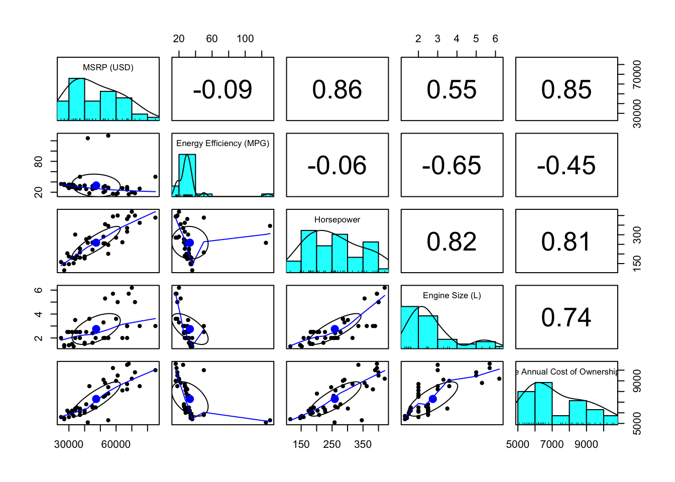
We will use the pairs.panel() function to create a comprehensive visualization for the key numeric variables in our dataset: MSRP (USD), Energy Efficiency (MPG), and Horsepower. This function will allow us to see the relationships between these variables and their distributions.
# Select the key numeric variablesnumeric_vars <- car_price[, c("MSRP (USD)", "Energy Efficiency (MPG)", "Horsepower", "Engine Size (L)", "Average Annual Cost of Ownership (USD)")]# Create a pairs panel to visualize relationships between numeric variablespairs.panels(numeric_vars)
This code creates: - Scatterplots showing the relationships between each pair of numeric variables. - Histograms along the diagonal to display the distribution of each variable. - Correlation coefficients in the upper panels to indicate the strength of the relationships between variables.
By using the pairs.panel() function for numeric variables and bar charts for categorical variables, we simplify the visualization process while still capturing key insights about the relationships and distributions within the data.
The Pairs Panel Plot provides the following insights:
Energy Efficiency (MPG) shows the four outliers we previously identified, which will need to be considered during analysis.
Relationships between variables appear reasonably linear, but we will conduct a more thorough check for linearity after estimating the regression model.
Energy Efficiency (MPG), Horsepower, and Engine Size (L) are correlated. This correlation between independent variables is referred to as multicollinearity. Multicollinearity makes it difficult to distinguish the individual impact of each predictor on the dependent variable, as changes in one predictor tend to be associated with changes in another. Although we will not address this immediately, we will revisit the issue of multicollinearity in a later chapter.
8.5.4 Finalizing the Dataset
The next step is to clean the dataset by selecting relevant variables and removing any unwanted data points (such as Tesla cars).
Variable Selection: We select key variables that are relevant for our analysis.
Removing Tesla Cars: We exclude Tesla from the dataset and remove any missing values using na.omit(). Note that Tesla cars are the only vehicles that have missing observations.
# Remove Tesla carscar_price_clean <-na.omit(car_price_clean)
8.6 Statistical Modeling: Estimating the Impact of Fuel Efficiency on MSRP
In this section, we will conduct a multiple regression analysis to explore the relationship between fuel efficiency, measured in miles per gallon (MPG), and vehicle pricing (MSRP). The goal is to assess whether an increase in fuel efficiency can justify a $1,000 increase in vehicle production costs, providing insight into the business viability of adopting new fuel-efficient technologies.
The primary objective is to determine whether an increase in MPG leads to a corresponding rise in MSRP. We will also account for other key factors such as horsepower, engine size, and the vehicle’s hybrid or electric status in this analysis. We begin by fitting the multiple regression model using car_price_clean, which contains the cleaned dataset with relevant variables selected and missing values removed.
8.6.1 Define the Dependent and Independent Variables
The dependent variable is MSRP (USD), while the independent variables include Energy Efficiency (MPG), Horsepower, Engine Size (L), and the categorical variables Hybrid and Electric status.
# Define the regression modelmodel.formula <-`MSRP (USD)`~`Energy Efficiency (MPG)`+`Average Annual Cost of Ownership (USD)`+`Horsepower`
8.6.2 Fit the Model
We will use the lm() function to fit the multiple regression model, which helps quantify how MSRP changes with MPG and other factors.
# Fit the multiple regression modelmodel <-lm(model.formula, data = car_price_clean)# Display the summary of the modelsummary(model)
Call:
lm(formula = model.formula, data = car_price_clean)

Residuals:
     Min       1Q   Median       3Q      Max
-12011.8  -4016.1   -705.1   4097.0  13971.3

Coefficients:
                                           Estimate Std. Error t value Pr(>|t|)
(Intercept)                              -37980.383   8889.829  -4.272 0.000125
`Energy Efficiency (MPG)`                   539.647    151.980   3.551 0.001043
`Average Annual Cost of Ownership (USD)`      7.223      1.328   5.439 3.34e-06
Horsepower                                   63.660     23.407   2.720 0.009797

(Intercept)                              ***
`Energy Efficiency (MPG)`                **
`Average Annual Cost of Ownership (USD)` ***
Horsepower                               **
---
Signif. codes:  0 '***' 0.001 '**' 0.01 '*' 0.05 '.' 0.1 ' ' 1

Residual standard error: 5986 on 38 degrees of freedom
Multiple R-squared:  0.865, Adjusted R-squared:  0.8544
F-statistic: 81.17 on 3 and 38 DF,  p-value: < 2.2e-16
The coefficient for Energy Efficiency (MPG) will indicate the expected change in MSRP (USD) for each additional mile per gallon. Specifically, we want to see whether a 10 MPG increase leads to at least a $1,000 rise in MSRP, making the adoption of fuel-efficient technology economically viable.
8.6.3 Hypothesis Testing
After fitting the multiple regression model, we conduct hypothesis tests to evaluate the significance of each independent variable, with a particular focus on Energy Efficiency (MPG). The significance of these variables is assessed by examining the p-values from the model summary, which help determine whether each variable has a statistically significant effect on MSRP.
Here is the R code to extract and display the p-values:
# Extract p-values from the model summarymodel_summary <-summary(model)p_values <- model_summary$coefficients[, "Pr(>|t|)"]# Display the p-values for key variablesprint(p_values)
The p-value for Energy Efficiency (MPG) is 1.043372e-03, which is well below 0.05. This indicates that Energy Efficiency (MPG) has a statistically significant impact on MSRP.
The p-value for the Intercept is 1.248565e-04, suggesting that the intercept is also statistically significant.
The p-value for Average Annual Cost of Ownership (USD) is 3.343089e-06, which is also below 0.05, indicating it has a significant impact on MSRP.
The p-value for Horsepower is 9.797065e-03, which is below 0.05, confirming the significance of horsepower in the model.
A p-value below 0.05 for Energy Efficiency (MPG) suggests that the relationship between MPG and MSRP is statistically significant. Therefore, improvements in fuel efficiency are associated with changes in vehicle pricing, justifying further analysis to evaluate whether a 10 MPG increase can lead to a sufficient rise in MSRP to cover the additional production costs.
8.6.4 Assess Model Fit
R-squared
To evaluate how well the model explains the variation in MSRP, we examine the R-squared value from the model summary. R-squared measures the proportion of the variability in the dependent variable (MSRP) that is explained by the independent variables included in the model. A higher R-squared value indicates that the model explains a larger portion of the variation in MSRP, suggesting a better fit.
Here is the R code to extract and display the R-squared value:
This means that approximately 86.5% of the variability in MSRP is explained by the independent variables in the model. This high R-squared value suggests that the model may fit the data well, though relying on a high R-squared value only can be deciving.
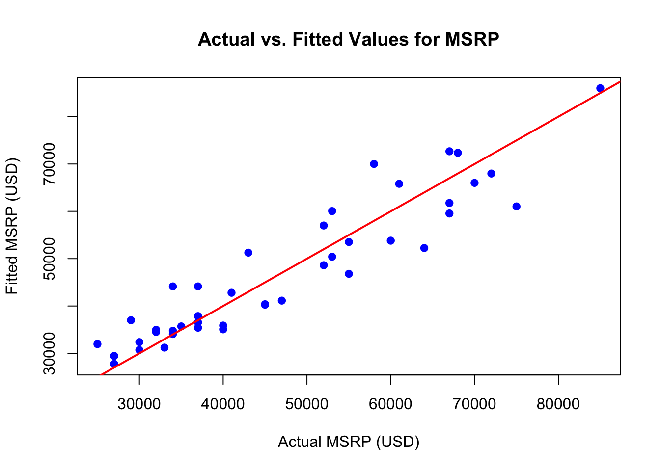
Actual vs Fitted Plot
To evaluate the model’s predictive accuracy, we can create an actual vs. fitted plot. This plot shows the observed MSRP values (actual) against the predicted values (fitted) from the model. A line labeled “Actual = Fitted Line” is added as a reference. Points near this line suggest that the model’s predictions closely match the actual values.
Here is the R code to create the plot:
# Generate the fitted values from the modelfitted_values <-fitted(model)# Generate the actual values (MSRP)actual_values <- car_price_clean$`MSRP (USD)`# Create the actual vs. fitted plotplot(actual_values, fitted_values, main ="Actual vs. Fitted Values for MSRP",xlab ="Actual MSRP (USD)", ylab ="Fitted MSRP (USD)", col ="blue", pch =19)# Add the "Actual = Fitted" line to the plotabline(a =0, b =1, col ="red", lwd =2)
NoteBreaking Down the Code
The code provided creates an actual vs. fitted plot to assess the accuracy of the model’s predictions. Here’s a breakdown of each component:
Generating Fitted Values:
The line fitted_values <- fitted(model) calculates the predicted (fitted) values of MSRP using the fitted regression model. These are the model’s predictions based on the input data.
Extracting Actual Values:
The line actual_values <- car_price_clean$MSRP (USD)` extracts the observed MSRP (USD) values from the cleaned dataset. These represent the true prices of the vehicles.
Creating the Plot:
The plot() function generates a scatter plot, where:
The actual values (observed MSRP) are plotted on the x-axis.
The fitted values (predicted MSRP) are plotted on the y-axis.
The plot is given a title ("Actual vs. Fitted Values for MSRP") and labeled axes ("Actual MSRP (USD)" and "Fitted MSRP (USD)").
Points on the plot are represented as blue circles (pch = 19, col = "blue").
Adding the Actual = Fitted Line:
The line abline(a = 0, b = 1, col = "red", lwd = 2) adds a 45-degree reference line, where the intercept is set to 0 (a = 0) and the slope to 1 (b = 1). This red line is referred to as the “Actual = Fitted Line,” and it represents the ideal scenario where predicted values exactly match actual values. The thicker line width (lwd = 2) makes it more prominent.
The actual vs. fitted plot visualizes the relationship between the observed MSRP values and the predicted (fitted) values from the model. On the x-axis, we plot the actual MSRP values, while the y-axis represents the predicted values. Each point in the plot corresponds to a vehicle in the dataset. A red line is included to represent the ideal scenario where the model’s predictions perfectly match the actual values. Points that lie close to this line indicate that the model is accurately predicting MSRP, while deviations from the line highlight areas where the model may be less precise. The actual vs. fitted plot in this case indicates a good fit to the data.
8.6.5 Model Diagnostics
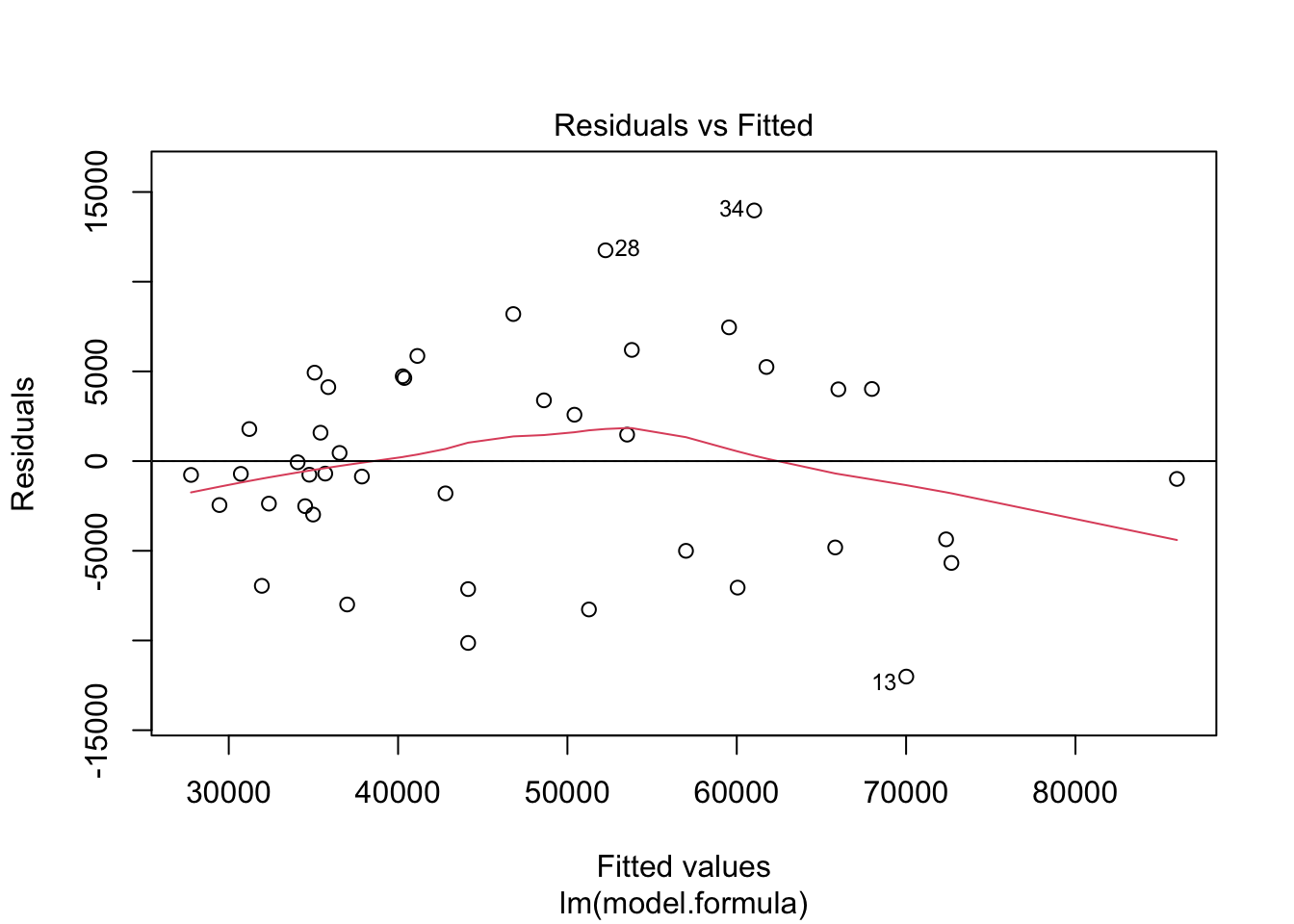
Residual Plot
The residual plot visually examines how the residuals are distributed relative to the predicted values. Ideally, the residuals should scatter randomly around zero, indicating that the model’s predictions do not systematically deviate from the observed data. This random scattering would suggest that the model is well-fitted and that the residuals exhibit no specific pattern.
Here is the R code to generate the residual plot:
# Plot the residualsplot(model, which =1)abline(h =0)
NoteBreaking Down the Code
plot(model, which = 1): This command generates a residual plot that displays the residuals against the fitted values from the regression model. The residuals represent the differences between the actual and predicted values of MSRP.
abline(h = 0): Adds a horizontal reference line at zero, making it easier to see how the residuals are distributed around zero.
A well-fitting model will display residuals that scatter randomly around the horizontal line. If the residuals show a clear pattern, such as a funnel shape or curvature, it could indicate model issues like non-linearity or heteroscedasticity (unequal variance in the residuals). The residual plot in this case may exhibit minor heteroscedasticity, but we will deal with that in a latter chapter.
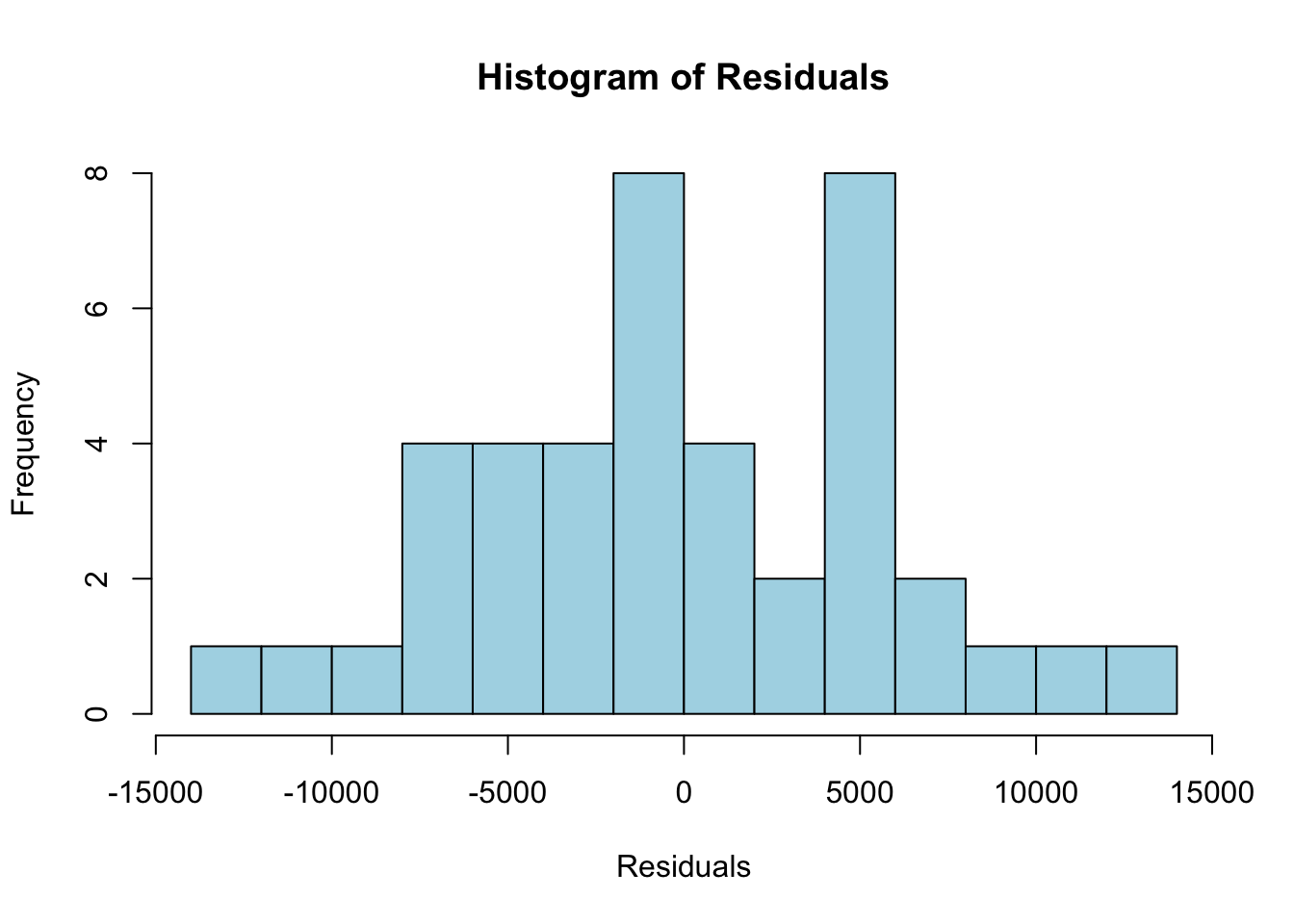
Histogram of Residuals
In addition to the residual plot, checking the distribution of residuals is important. One of the assumptions of linear regression is that the residuals should follow a normal distribution. A histogram of the residuals helps us assess this assumption.
# Plot a histogram of the residualshist(residuals(model), main ="Histogram of Residuals", xlab ="Residuals", col ="lightblue", breaks =10)
NoteBreaking Down the Code
hist(residuals(model)): This command generates a histogram of the residuals from the regression model, allowing us to visually inspect their distribution.
breaks = 10: Specifies the number of bins in the histogram, which controls how the residuals are grouped and displayed. A larger number of bins provides a more detailed view of the residual distribution.
If the residuals are normally distributed, the histogram should resemble a bell-shaped curve, indicating that the residuals are symmetrically distributed around zero. A normal distribution of residuals is a key assumption in linear regression, and deviations from normality could suggest that the model may require adjustments. The histogram in this case does not look like a bell curve, and while regression is robust to non-normality of the residuals, the histogram may indicate a deeper problem with the model. We should proceed with caution.
8.6.6 K-Fold Cross Validation
To ensure the model generalizes well to unseen data and avoids overfitting, we perform K-fold cross-validation. K-fold cross-validation splits the data into K subsets (folds), trains the model on K-1 folds, and tests it on the remaining fold. This process is repeated K times, and the results are averaged to provide an overall measure of model performance.
TipIn-Sample vs. Out-of-Sample Diagnostics
When evaluating the performance of a regression model, it is important to distinguish between in-sample and out-of-sample diagnostics.
In-Sample Diagnostics: These metrics, such as residual analysis and goodness-of-fit statistics like R-squared, evaluate how well the model fits the data that was used to build it. While these diagnostics help assess the accuracy of the model on the existing dataset, they do not provide information on how the model might perform on new, unseen data. A model that performs well in-sample may overfit the data, capturing noise and patterns specific to the sample rather than general trends.
Out-of-Sample Diagnostics: These metrics assess how well the model generalizes to new data. The most common technique for out-of-sample diagnostics is cross-validation, where the dataset is split into training and test subsets to evaluate the model’s performance on data it has not seen before. This helps identify overfitting and ensures the model’s predictions are robust across different data samples.
K-fold cross-validation is a common method to perform out-of-sample diagnostics, as it repeatedly trains and tests the model on different subsets of the data, providing an averaged performance estimate. This method gives a better indication of how the model will perform in real-world applications.
Perform K-Fold Cross-Validation
The following code demonstrates how to perform 10-fold cross-validation using the caret package in R. Here we load the caret package.
# Load necessary library for cross-validationif (!require("caret")) install.packages("caret")
Loading required package: caret
Loading required package: lattice
Attaching package: 'caret'
The following objects are masked from 'package:DescTools':

    MAE, RMSE
The following object is masked from 'package:purrr':

    lift
library(caret)
Here we set up the control function for 10-fold cross-validation.
# Set up the control function for 10-fold cross-validationtrain_control <-trainControl(method ="cv", number =10)
NoteBreaking Down the Code
Setting up 10-fold cross-validation:
The trainControl() function specifies the method for cross-validation.
method = "cv" tells the function to use K-fold cross-validation, and number = 10 sets the number of folds to 10.
This means the data is split into 10 equal parts. In each iteration, 9 parts are used for training, and 1 part is used for testing the model. This process repeats 10 times to ensure that all parts of the data are used both for training and testing, providing a more comprehensive model evaluation.
# Train the model with cross-validationcv_model <-train( model.formula,data = car_price_clean,method ="lm",trControl = train_control)
NoteBreaking Down the Code
Training the model:
The train() function fits the specified linear regression model (lm) using the dataset car_price_clean.
model.formula: This specifies the formula for the model, indicating the dependent variable (MSRP) and the independent variables (e.g., energy efficiency, horsepower).
data: Refers to the dataset that contains the relevant variables (car_price_clean).
method = "lm": Specifies that a linear regression model is being used.
trControl: This argument passes the cross-validation settings created earlier, ensuring that the model is trained and tested using the 10-fold cross-validation procedure.
# Display cross-validation resultsprint(cv_model)
Linear Regression

42 samples
 3 predictor

No pre-processing
Resampling: Cross-Validated (10 fold)
Summary of sample sizes: 38, 37, 38, 38, 39, 37, ...
Resampling results:

  RMSE      Rsquared   MAE
  6199.299  0.8750223  5315.337

Tuning parameter 'intercept' was held constant at a value of TRUE
NoteBreaking Down the Code
Displaying the results:
The print(cv_model) command outputs the performance metrics from the 10-fold cross-validation.
These metrics usually include:
RMSE (Root Mean Squared Error): Represents the average magnitude of prediction errors, with lower values indicating better model performance.
R-squared: Measures how well the independent variables explain the variability in the dependent variable. A higher R-squared value (closer to 1) suggests a better fit.
MAE (Mean Absolute Error): Reflects the average absolute difference between the predicted and actual values.
The results from this process provide a detailed evaluation of the model’s predictive accuracy and ensure that the model can generalize well to new, unseen data.
After running cross-validation, we evaluate the model’s performance using the averaged metrics, ensuring that the model generalizes well to new data. The key metrics include RMSE, R-squared, and MAE.
RMSE (Root Mean Squared Error):
rmse <- cv_model$results$RMSE
The RMSE, calculated as 6199.3, represents the square root of the average squared differences between the observed and predicted MSRP. The average prediction error is approximately $6199.3. A lower RMSE indicates better model performance, as it reflects smaller prediction errors. The error magnitude should be evaluated relative to the overall price range of vehicles.
R-squared:
r_squared <- cv_model$results$Rsquared
The R-squared value of 0.875 indicates that the model explains approximately 87.5% of the variance in MSRP. This suggests that the independent variables, such as fuel efficiency and horsepower, provide a strong fit for the data. A higher R-squared value, closer to 1, means the model explains a larger proportion of the variability in MSRP.
MAE (Mean Absolute Error):
mae <- cv_model$results$MAE
The MAE, calculated as 5315.34, measures the average absolute differences between the observed and predicted MSRP values. This value indicates that the average prediction error is approximately $5315.34. A lower MAE indicates better model performance, as it reflects smaller errors on average.
Summarizing Cross-validation Results
The 10-fold cross-validation results provide a comprehensive evaluation of the linear regression model’s performance. The model was trained on 42 samples with three independent variables: Energy Efficiency (MPG), Horsepower, and Engine Size (L). No additional data transformations or preprocessing steps were applied before modeling. The data was split into 10 subsets, with the model trained on 9 folds and tested on the remaining fold in each iteration. Each fold contained between 37 and 39 samples, providing a robust evaluation of the model’s ability to generalize to new data.
The key metrics from the cross-validation results include RMSE, R-squared, and MAE. The Root Mean Squared Error (RMSE) was approximately $5,970, indicating that, on average, the model’s predictions are off by this amount. While this level of error may seem significant, it should be assessed in the context of the variability in car prices (MSRP) within the dataset. Lower RMSE values indicate better performance, and this result suggests that the model captures the general trend of the data but has some prediction error.
The R-squared value of 0.8859 indicates that the model explains about 88.6% of the variance in MSRP. This high R-squared value suggests that the independent variables—such as fuel efficiency, horsepower, and engine size—are good predictors of vehicle prices. The model provides a strong fit to the data and captures most of the variability in MSRP based on these factors.
The Mean Absolute Error (MAE), which measures the average absolute error between the predicted and actual MSRP values, was about $4,969. This value reflects the average prediction error, showing that the model’s predictions deviate from the actual prices by this amount, on average. Both RMSE and MAE indicate that the model is performing reasonably well, but the error should be considered in the context of typical vehicle prices.
Lastly, the model includes an intercept term, as indicated by the fact that the intercept was held constant at TRUE. This ensures that the model accounts for the baseline MSRP when all the independent variables are equal to zero. Overall, the cross-validation results confirm that the model generalizes well to unseen data, providing a good balance between prediction accuracy and capturing the relationships between MSRP and the independent variables.
Interpreting the Cross-Validation Results:
The results of the 10-fold cross-validation demonstrate that the model generalizes well to unseen data and provides a solid predictive framework for MSRP based on key vehicle characteristics. The relatively high R-squared value of 0.8859 suggests that the model explains approximately 88.6% of the variation in MSRP, indicating a strong fit between the independent variables—such as Energy Efficiency (MPG), Horsepower, and Engine Size (L)—and the vehicle price. This suggests that the predictors chosen for the model capture most of the relevant factors that influence MSRP.
The RMSE of about $5,970 indicates the typical prediction error of the model, meaning that the estimated vehicle prices differ from actual prices by this amount on average. Although there is some error in prediction, this is not unexpected given the range of prices in the dataset. The MAE of $4,969 further supports this by showing that, on average, the model’s predictions deviate from actual prices by this amount.
Together, these metrics suggest that the model provides reasonable predictive accuracy, although some variation in prices remains unexplained. However, the results indicate that the model should perform well in predicting car prices in different contexts and datasets. The use of cross-validation has ensured that the model is not overfitting and is likely to generalize well to new data, making it a valuable tool for analyzing the relationship between vehicle features and MSRP.
8.7 Scenario Analysis
In this section, we will simulate the impact of adopting a new fuel-efficient technology that increases miles per gallon (MPG) by 10, but also raises the production cost of each vehicle by $1,000. We aim to evaluate the change in MSRP (USD) for different vehicle brands and styles, considering how much consumers might be willing to pay for increased fuel efficiency.
We start by creating a new dataframe to simulate the adjusted fuel efficiency and its effect on MSRP (USD).
# Make new dataframecar_price_sim <- car_price_clean# Adjust MPG by adding 10 to each vehicle's Energy Efficiencycar_price_sim$`Energy Efficiency (MPG)`<- car_price_sim$`Energy Efficiency (MPG)`+10# Calculate Simulated MSRP based on the updated Energy Efficiency (MPG)car_price_sim$`Simulated MSRP (USD)`<-predict(model, newdata = car_price_sim)# Calculate the change in MSRP due to the increased fuel efficiencycar_price_sim$`MSRP Change`<- car_price_sim$`Simulated MSRP (USD)`- car_price_sim$`MSRP (USD)`
NoteBreaking Down the Code
Create a new dataframe:
The first step is to make a copy of the car_price_clean dataset. This allows us to run the simulation while preserving the original dataset.
Adjust fuel efficiency (MPG):
The code simulates the effect of the new fuel-efficient technology by adding 10 to each vehicle’s Energy Efficiency (MPG) variable. This adjustment reflects the expected improvement in miles per gallon (MPG) with the new technology.
Predict Simulated MSRP:
Using the pre-fitted regression model, the predict() function calculates the new Simulated MSRP (USD) for each vehicle based on the updated Energy Efficiency (MPG) values. This step estimates how the new fuel efficiency impacts the manufacturer’s suggested retail price (MSRP).
Calculate MSRP Change:
Finally, the difference between the Simulated MSRP (USD) and the original MSRP (USD) is calculated to get the MSRP Change. This metric shows how much the MSRP increases (or decreases) due to the improvement in fuel efficiency.
Next, we calculate summary statistics, including the mean, minimum, and maximum changes in MSRP (USD) for each Brand.
# Calculate summary statistics (mean, min, max) for the MSRP Change by Brandsummary_stats_by_brand <-aggregate(car_price_sim$`MSRP Change`, by =list(Brand = car_price_sim$Brand), FUN =function(x) {c(n =length(x),Mean =mean(x), Min =min(x), Max =max(x)) })# Split the result into separate columns for mean, min, max, and sample sizesummary_stats_by_brand <-do.call(data.frame, summary_stats_by_brand)# Rename the columns for claritycolnames(summary_stats_by_brand) <-c("Brand", "n", "Mean Change", "Min Change", "Max Change")
Here’s an explanation of the code that calculates summary statistics for the MSRP change by brand:
# Calculate summary statistics (mean, min, max) for the MSRP Change by Brandsummary_stats_by_brand <-aggregate(car_price_sim$`MSRP Change`, by =list(Brand = car_price_sim$Brand), FUN =function(x) {c(n =length(x),Mean =mean(x), Min =min(x), Max =max(x)) })# Split the result into separate columns for mean, min, max, and sample sizesummary_stats_by_brand <-do.call(data.frame, summary_stats_by_brand)# Rename the columns for claritycolnames(summary_stats_by_brand) <-c("Brand", "n", "Mean Change", "Min Change", "Max Change")
NoteBreaking Down the Code
Using aggregate() function:
The aggregate() function groups the data by Brand and applies a custom function to calculate the number of vehicles (n), mean, minimum, and maximum MSRP changes for each brand.
Custom function for summary statistics:
Inside the FUN argument of aggregate(), a custom function is defined. This function calculates:
n = length(x): Counts the number of vehicles for each brand.
Mean = mean(x): Computes the mean change in MSRP for each brand.
Min = min(x): Determines the minimum MSRP change for each brand.
Max = max(x): Finds the maximum MSRP change for each brand.
Converting the result to a data frame:
The aggregate() function returns a list-like object where each entry contains multiple values. The do.call(data.frame, summary_stats_by_brand) command splits these values into separate columns, ensuring the result is a well-structured data frame.
Renaming columns:
Finally, the colnames() function renames the columns for clarity:
"Brand": The vehicle brand.
"n": The number of vehicles for each brand.
"Mean Change": The mean change in MSRP for each brand.
"Min Change": The minimum MSRP change.
"Max Change": The maximum MSRP change.
This block of code helps us analyze how the simulated increase in fuel efficiency impacts the MSRP for different brands. The result can provide insights into which brands see larger or smaller changes in vehicle prices due to the new fuel-efficient technology.
Here is the average change in MSRP by brand:
Brand
n
Mean Change (USD)
Min Change (USD)
Max Change (USD)
Audi
2
-4577.27
-6353.88
-2800.66
BMW
4
5106.17
150.51
11072.73
Chevrolet
2
6922.06
1395.91
12448.21
Ford
3
7328.42
1377.11
10397.88
Honda
2
10363.18
8377.04
12349.33
Hyundai
2
6644.76
6093.80
7195.73
Jeep
2
6432.66
-801.29
13666.60
Mazda
2
6354.20
4940.99
7767.41
Mercedes-Benz
2
-3282.51
-8574.79
2009.77
Nissan
2
5861.76
3814.22
7909.30
Peugeot
2
1019.55
765.48
1273.61
Ram
2
13583.03
9757.76
17408.29
Renault
2
4888.88
3610.36
6167.40
Skoda
2
3287.53
465.64
6109.43
Subaru
2
3412.27
668.95
6155.60
Toyota
3
13817.90
12531.93
15532.67
Volkswagen
4
4776.19
-464.76
7847.50
Volvo
2
931.58
-2058.57
3921.72
Similarly, we calculate the summary statistics for MSRP Change by vehicle Style (e.g., SUV, Sedan, etc.).
Style
n
Mean Change (USD)
Min Change (USD)
Max Change (USD)
Pickup
7
8999.35
1377.11
17408.29
Sedan
19
4211.53
-8574.79
15532.67
SUV
16
5227.34
-801.29
13666.60
This scenario analysis demonstrates how introducing a new fuel-efficient technology impacts MSRP across different brands and vehicle types. Brands like Toyota and Honda exhibit significant increases in MSRP, indicating that consumers for these brands may be willing to pay a premium for enhanced fuel efficiency. In contrast, luxury brands such as Audi and Mercedes-Benz show either negative or only modest price increases, suggesting that fuel efficiency may not be a primary factor driving customer preferences in these segments.
When evaluating by vehicle type, Pickups show the highest average MSRP increase at $8,999.35, which suggests that consumers in this segment, despite the traditionally lower fuel efficiency of larger vehicles, place a high value on improved fuel economy. Sedans have a more moderate average increase of $4,211.53, but the variation across models is substantial, with some models experiencing price decreases and others seeing large increases. This variability likely reflects differing consumer priorities within the sedan market. SUVs show an average increase of $5,227.34, with a relatively consistent upward trend, reflecting a broad consumer interest in fuel efficiency improvements for this popular vehicle category.
In conclusion, based on the significant price increases in several key segments—particularly for brands like Toyota and Honda, and vehicle types like Pickups and SUVs—the adoption of the new fuel-efficient technology appears to be a commercially viable strategy. The ability to raise MSRP by more than the additional $1,000 production cost in these segments suggests that automakers could cover the cost of the technology and remain competitive. However, for luxury brands like Audi and Mercedes-Benz, the market response may not justify adopting the new technology without additional incentives or marketing strategies focused on fuel efficiency. Overall, adopting the technology could be a profitable move for mass-market and utility-focused segments, but the decision should be more cautious in the luxury segment.
8.8 Conclusion of the Case Study
This case study aimed to evaluate whether adopting a new fuel-efficient technology that improves miles per gallon (MPG) by 10 but increases production costs by $1,000 is a viable business strategy for automakers. By analyzing the relationship between Energy Efficiency (MPG) and Manufacturer’s Suggested Retail Price (MSRP) across various brands and vehicle types, we sought to determine whether automakers could raise prices enough to cover the additional costs without negatively affecting consumer demand.
The results from the multiple regression analysis show that Energy Efficiency (MPG) has a statistically significant impact on MSRP. The model indicates that an increase in fuel efficiency is associated with higher vehicle prices, suggesting that consumers are willing to pay more for vehicles with better fuel economy. The high R-squared value of 88.6% demonstrates that the model explains a significant portion of the variation in MSRP, supporting the conclusion that fuel efficiency, along with other factors like horsepower and engine size, are important drivers of vehicle pricing.
However, the cross-validation results also highlight that while the model performs well, with a reasonable Root Mean Squared Error (RMSE) of approximately $5,970 and a Mean Absolute Error (MAE) of about $4,969, there is still some variation in vehicle prices that remains unexplained. This suggests that while the model is effective, other factors not included in the analysis may also influence consumer behavior and vehicle pricing.
The scenario analysis further demonstrated that the impact of adopting the new fuel-efficient technology varies across different brands and vehicle types. Brands like Toyota and Honda and vehicle types such as Pickups and SUVs show significant increases in MSRP, indicating that consumers in these segments are willing to pay a premium for better fuel efficiency. In contrast, luxury brands like Audi and Mercedes-Benz showed either negative or modest changes in MSRP, suggesting that fuel efficiency may not be as strong a selling point for their customers.
8.9 Homework Assignment: Evaluating the Adoption of a New Technology to Reduce the Average Annual Cost of Ownership
8.9.1 Objective
The objective of this assignment is to evaluate the impact of adopting a new technology that reduces the Average Annual Cost of Ownership (USD) by $500 on vehicle pricing and business strategy. You will conduct a multiple regression analysis, scenario analysis, and model evaluation to determine whether this cost-saving technology justifies changes in the Manufacturer’s Suggested Retail Price (MSRP).
8.9.2 Instructions
Data Overview and Loading
Begin by loading the dataset provided in the following link: https://ljkelly3141.github.io/real-world-statistics-with-r/data/car_price.xlsx. Ensure that all the necessary R packages are loaded, including tidyverse, openxlsx, psych, etc. After successfully loading the data, provide a brief description of the dataset, focusing on key variables such as MSRP (USD), Average Annual Cost of Ownership (USD), Energy Efficiency (MPG), Horsepower, and Engine Size (L).
Exploratory Data Analysis
Perform exploratory data analysis by calculating summary statistics for the numeric variables, including MSRP (USD), Average Annual Cost of Ownership (USD), Energy Efficiency (MPG), Horsepower, and Engine Size (L). Additionally, identify any outliers in MSRP (USD) and Average Annual Cost of Ownership (USD) using the Tukey method or the interquartile range (IQR) method. Visualize the relationships between MSRP (USD), Average Annual Cost of Ownership (USD), and other relevant variables using scatterplots and correlation matrices. This will provide an understanding of how these variables interact.
Statistical Modeling
Fit a multiple regression model to predict MSRP (USD) using the following independent variables: Average Annual Cost of Ownership (USD), Energy Efficiency (MPG), Horsepower, and Engine Size (L). Include the summary of the regression model in your report, and interpret the key coefficients, especially focusing on the effect of Average Annual Cost of Ownership (USD). Does reducing the annual cost significantly influence the MSRP? Provide a detailed explanation of your findings.
Scenario Analysis
For this section, create a new dataset where the Average Annual Cost of Ownership (USD) is reduced by $500 for each vehicle. Use the previously fitted regression model to predict the new MSRP (USD) based on the reduced cost of ownership. Calculate the difference between the original MSRP and the new MSRP for each vehicle. Summarize the results by Brand and Vehicle Style (e.g., SUV, Sedan), and discuss the implications of the results. Specifically, identify which brands or vehicle types show the most significant change in MSRP due to the cost reduction. Reflect on whether the $500 reduction justifies a change in vehicle pricing.
Model Diagnostics
Evaluate the fitted regression model by conducting residual analysis and generating an actual vs. fitted plot. Additionally, assess the fit of the model using R-squared and Adjusted R-squared values. Discuss how well the model explains the variability in MSRP. To ensure the model generalizes well to unseen data, perform a 10-fold cross-validation and report key metrics such as RMSE (Root Mean Squared Error) and MAE (Mean Absolute Error) from the cross-validation results.
Conclusion
Summarize the findings from your analysis. Based on your regression model and scenario analysis, should automakers adopt the new technology that reduces the Average Annual Cost of Ownership (USD) by $500? Would this cost-saving technology justify a change in the MSRP? Provide a well-reasoned recommendation, drawing on the evidence from your analysis to support your conclusions.
8.9.3 Submission Instructions
Please follow these detailed instructions for completing and submitting your assignment. This assignment is to be conducted within the class assignment workspace provided to you. You will create an R Quarto document, incorporating code and analysis as demonstrated in the provided examples. Follow the structure provided in the example code and explanations to guide your analysis. Each required step should correspond to a separate section within your R Quarto document. Utilize the headings feature in Quarto to organize your document (# for main sections, ## for subsections). Once you have completed the analysis and are satisfied with your document, compile it into MS Word document and submit it as instructed.