6 Case Study: Simple Linear Regression
PRELIMINARY AND INCOMPLETE
6.1 Introduction
In this case study, we will explore how simple linear regression can be used to analyze car market data. Specifically, we aim to model the relationship between a vehicle’s horsepower and its energy efficiency, measured in miles per gallon (MPG). This analysis can provide valuable insights into optimizing vehicle performance, balancing the trade-offs between power and fuel economy, and understanding how engine characteristics impact energy efficiency.
6.2 Objective
The primary objective of this case study is to demonstrate how to use simple linear regression to predict energy efficiency (MPG) based on horsepower. Through this process, we will: - Introduce the fundamental concepts of regression analysis. - Highlight the steps involved in building, diagnosing, and refining a regression model. - Investigate potential outliers and assess their impact on the model’s validity.
6.3 Workflow of Regression Analysis
The workflow for performing a regression analysis typically involves the following key steps:
Data Preparation: The first step is loading and preparing the dataset, which involves selecting relevant variables and handling missing or incomplete data. For this case study, we will focus on two key variables: horsepower (the independent variable) and energy efficiency (MPG) (the dependent variable).
Exploratory Data Analysis (EDA): Next, we conduct an initial examination of the data to understand relationships and potential trends. This includes creating scatter plots to visualize the relationship between the variables and identifying any potential outliers that could affect the analysis.
Model Building: Once the data has been explored, we move on to fitting a simple linear regression model. This involves estimating the coefficients of the regression equation, which quantifies the relationship between the independent and dependent variables.
Model Diagnostics: After building the model, it is essential to check its assumptions and evaluate its performance. This step involves analyzing residuals (the difference between observed and predicted values) to ensure that the model is appropriate. We will also check the normality of residuals to confirm that the model assumptions are met.
Model Refinement: If necessary, we refine the model by removing outliers, transforming variables, or considering alternative model structures to improve the fit and predictive power.
Interpretation and Reporting: Finally, we interpret the results of the regression model, summarizing the key findings and providing actionable insights. For this case study, we will determine how horsepower influences energy efficiency and highlight any outliers that may affect this relationship.
Through this case study, you will learn how to apply simple linear regression to real-world car market data, diagnose potential issues with the model, and interpret the results for informed decision-making.
6.4 Dataset Overview
The dataset used in this case study contains a mixture of both numeric and categorical variables, simulating realistic vehicle data that might be used by manufacturers and analysts. This data, while simulated, is designed to represent key factors in vehicle performance, customer preferences, and cost.
The variables in the dataset cover a wide range of attributes, from technical specifications such as horsepower and engine size to customer-related data like satisfaction ratings and cost of ownership. These variables allow for a detailed analysis of the relationships between various vehicle characteristics and outcomes such as energy efficiency.
Below is an overview of the relevant variables for this case study:
| Variable Name | Description | Data Type | Categorical Type |
|---|---|---|---|
Brand |
Manufacturer of the vehicle (e.g., Tesla, Toyota, Ford) | Categorical | Nominal |
Model |
Specific model of the vehicle (e.g., Camry, Model 3) | Categorical | Nominal |
Trim |
Version or package level of the vehicle model | Categorical | Nominal |
Trim_Level |
Luxury or feature set of the vehicle (Base, Medium, Premium) | Categorical | Ordinal |
Style |
Body type of the vehicle (Sedan, SUV, Pickup) | Categorical | Nominal |
Size |
Size class of the vehicle (Compact, Midsize, Full-size) | Categorical | Ordinal |
MSRP (USD) |
Manufacturer’s Suggested Retail Price in U.S. dollars | Numeric | - |
Energy Efficiency (MPG) |
Fuel efficiency measured in miles per gallon (MPG) | Numeric | - |
Horsepower |
Power output of the vehicle, measured in horsepower (HP) | Numeric | - |
Engine Size (L) |
Engine displacement measured in liters | Numeric | - |
Customer Rating |
Customer satisfaction rating (out of 5 stars) | Numeric | - |
Safety Rating |
Safety rating based on crash test performance (1-5 stars) | Numeric | - |
Hybrid |
Whether the vehicle is a hybrid (Hybrid/Non-Hybrid) | Categorical | Nominal |
Electric |
Whether the vehicle is fully electric (Electric/Non-Electric) | Categorical | Nominal |
Four_Wheel_Drive |
Indicates if the vehicle has 4WD (4WD/2WD) | Categorical | Nominal |
Sunroof |
Whether the vehicle has a sunroof (Yes/No) | Categorical | Nominal |
Bluetooth |
Whether the vehicle has Bluetooth connectivity (Yes/No) | Categorical | Nominal |
Backup Camera |
Whether the vehicle has a backup camera (Yes/No) | Categorical | Nominal |
Main Market |
The primary market where the vehicle is sold (North America/Europe) | Categorical | Nominal |
Average Annual Cost of Ownership (USD) |
Estimated total annual cost of owning the vehicle in USD | Numeric | - |
In the next section, we will prepare the dataset for analysis, focusing on selecting the relevant columns and cleaning the data to ensure a robust regression model.
6.5 Data Loading and Preparation
In this section, we will load the necessary packages, import the dataset, and clean the data to prepare it for analysis. The dataset contains vehicle characteristics, including horsepower and energy efficiency, which will be the primary variables for our regression analysis. Additionally, we will leverage summary statistics to ensure that the dataset is properly structured and ready for modeling.
Note: Readers can download the dataset used in this analysis from https://ljkelly3141.github.io/real-world-statistics-with-r/data/car_price.xlsx.
6.5.1 Loading Necessary Packages
Before loading and cleaning the data, we need to install and load the required R packages for data handling and statistical analysis. The readxl package is used to read Excel files, while the psych package provides a variety of functions for data summary and descriptive statistics.
6.5.2 Loading and Cleaning Data
Once the packages are loaded, we proceed with importing the car dataset from an Excel file. After loading the data, we will clean it by selecting only the relevant columns (in this case, horsepower and energy efficiency) and removing any rows with missing values. Additionally, we will generate summary statistics to ensure the data is ready for analysis.
| Brand | Model | Trim | Trim Level | Style | Size | MSRP (USD) | Energy Efficiency (MPG) | Horsepower | Engine Size (L) | Customer Rating | Safety Rating | Hybrid | Electric | Four_Wheel_Drive | Sunroof | Bluetooth | Backup_Camera | Main Market | Average Annual Cost of Ownership (USD) |
|---|---|---|---|---|---|---|---|---|---|---|---|---|---|---|---|---|---|---|---|
| Toyota | Camry | LE | Base | Sedan | Midsize | 2.9e+04 | 32 | 203 | 2.5 | 4.5 | 5 | Non-Hybrid | Non-Electric | 2WD | Sunroof | Bluetooth | Backup Camera | North America | 6.2e+03 |
| Toyota | Camry | XSE | Medium | Sedan | Midsize | 3.4e+04 | 31 | 301 | 3.5 | 4.7 | 5 | Non-Hybrid | Non-Electric | 2WD | Sunroof | Bluetooth | Backup Camera | North America | 6.4e+03 |
| Toyota | Camry | Hybrid | Premium | Sedan | Midsize | 3.7e+04 | 50 | 208 | 2.5 | 4.8 | 5 | Hybrid | 2WD | Sunroof | Bluetooth | Backup Camera | North America | 5.8e+03 | |
| Ford | F-150 | XLT | Base | Pickup | Full-size | 5.2e+04 | 20 | 290 | 3.3 | 4.4 | 5 | Non-Hybrid | 4WD | Bluetooth | Backup Camera | North America | 9.1e+03 | ||
| Ford | F-150 | Lariat | Medium | Pickup | Full-size | 6.1e+04 | 18 | 400 | 5 | 4.6 | 5 | Non-Hybrid | 4WD | Sunroof | Bluetooth | Backup Camera | North America | 9.5e+03 | |
| Ford | F-150 | Platinum | Premium | Pickup | Full-size | 7.2e+04 | 18 | 400 | 5 | 4.8 | 5 | Non-Hybrid | 4WD | Sunroof | Bluetooth | Backup Camera | North America | 9.8e+03 |
# Select relevant columns: 'Brand', 'Model', 'Horsepower', and 'Energy Efficiency (MPG)'
car_data <- car_data[, c("Brand", "Model", "Horsepower", "Energy Efficiency (MPG)")]

# Remove rows with missing values
car_data <- na.omit(car_data)

# Display summary statistics of the selected data
describe(car_data, skew = FALSE, omit = TRUE)| vars | n | mean | sd | median | min | max | range | se |
|---|---|---|---|---|---|---|---|---|
| 3 | 44 | 259 | 84.8 | 255 | 115 | 420 | 305 | 12.8 |
| 4 | 44 | 33.2 | 22.1 | 29 | 16 | 130 | 114 | 3.33 |
Next, we will perform exploratory data analysis (EDA) to visualize the relationships between horsepower and energy efficiency, and identify any potential outliers.
6.6 Exploratory Data Analysis (EDA)
In this section, we will explore the relationship between horsepower and energy efficiency (MPG) through scatter plots. We will start by visualizing the raw data and then use the Tukey method to identify and highlight outliers. Afterward, we will remove the outliers and replot the data to reassess the relationship.
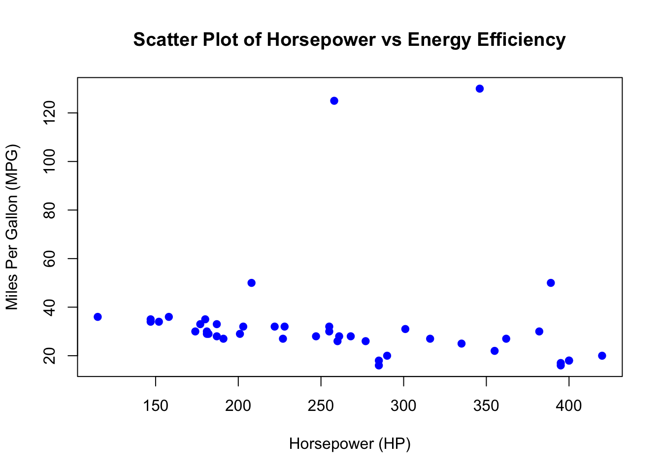
6.6.1 Initial Scatter Plot
We begin by creating a scatter plot to visualize the relationship between horsepower and energy efficiency (MPG) for the vehicles in the dataset.
6.6.2 Identifying and Highlighting Outliers (Tukey Method)
Next, we use the Tukey method to identify potential outliers in the Energy Efficiency (MPG) variable. The Tukey method defines outliers as values that fall outside of the interquartile range (IQR), specifically below Q1 - 1.5 * IQR or above Q3 + 1.5 * IQR.
# Calculate IQR and Tukey outlier thresholds
iqr <- IQR(car_data$`Energy Efficiency (MPG)`)
q1 <- quantile(car_data$`Energy Efficiency (MPG)`, 0.25)
q3 <- quantile(car_data$`Energy Efficiency (MPG)`, 0.75)
lower_bound <- q1 - 1.5 * iqr
upper_bound <- q3 + 1.5 * iqr

# Identify outliers
outliers_indices <- car_data$`Energy Efficiency (MPG)` < lower_bound |
                    car_data$`Energy Efficiency (MPG)` > upper_bound

# Scatter plot with outliers highlighted
plot(car_data$Horsepower, car_data$`Energy Efficiency (MPG)`,
     main = "Scatter Plot of Horsepower vs Energy Efficiency (Outliers Highlighted)",
     xlab = "Horsepower (HP)",
     ylab = "Miles Per Gallon (MPG)",
     pch = 19, col = "blue")

# Highlight outliers in red
points(car_data$Horsepower[outliers_indices],
       car_data$`Energy Efficiency (MPG)`[outliers_indices],
       col = "red",
       pch = 19)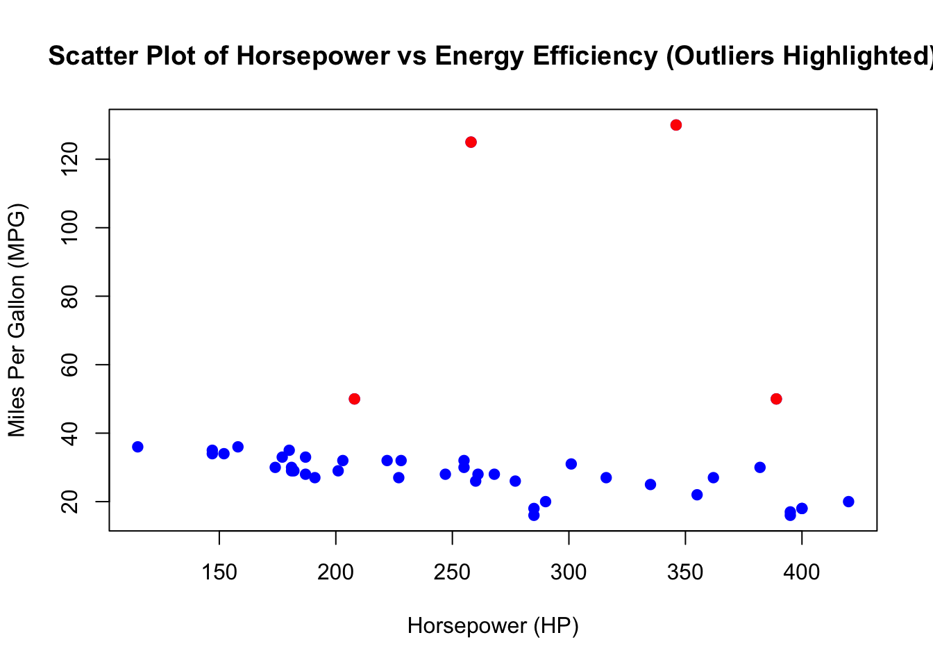
6.6.3 Identifying Outlier Car Makes and Models
After identifying the outliers in the dataset, it is useful to investigate which car makes and models are classified as outliers based on their Energy Efficiency (MPG) values. By looking at these vehicles, we can determine if certain types of cars (e.g., electric vehicles or high-performance cars) are consistently being flagged as outliers.
| Brand | Model | Horsepower | Energy Efficiency (MPG) |
|---|---|---|---|
| Toyota | Camry | 208 | 50 |
| Tesla | Model 3 | 258 | 125 |
| Tesla | Model 3 | 346 | 130 |
| BMW | X5 | 389 | 50 |
By examining the brands and models of the outlier vehicles, we can identify whether certain types of cars, such as electric vehicles (like the Tesla Model 3), might skew the analysis due to their different energy efficiency characteristics compared to traditional gasoline vehicles.
6.6.4 Strategies for Dealing with Outliers
Outliers can have a significant impact on the results of a regression analysis. They may skew the relationship between the variables, distort model parameters, or influence the overall interpretation of the data. When faced with outliers, it is essential to carefully consider how to handle them to ensure robust and meaningful results. Below are several strategies for dealing with outliers in a dataset like the one we are analyzing:
-
Remove Outliers (Trimming the Data) One common approach is to remove the outliers from the dataset. This method is appropriate when the outliers are extreme and clearly result from data entry errors or represent rare, atypical cases that do not fit the general trend.
Advantages:
- Simplifies the dataset by focusing only on the central trend.
- Can improve model accuracy by reducing the influence of extreme values.
Disadvantages:
- Risk of losing valuable information if the outliers represent valid but rare cases.
- Removal of outliers could bias the results if the outliers are systematically related to the outcome of interest.
In this case, removing vehicles such as the Tesla Model 3 (which has very high MPG) might give a clearer view of the relationship between horsepower and energy efficiency for traditional gasoline-powered vehicles.
-
Transform the Data Another strategy is to apply a mathematical transformation to the data, such as a log transformation, to reduce the influence of outliers. This can be particularly useful when the relationship between variables is non-linear or when the distribution of the data is skewed.
Advantages:
- Retains all data points, including outliers.
- Can make the relationship between variables more linear, improving the fit of a regression model.
Disadvantages:
- Interpretation of transformed variables can be less intuitive.
- Some outliers may still exert significant influence, even after transformation.
For example, applying a log transformation to energy efficiency (MPG) might reduce the impact of electric vehicles like the Tesla Model 3, which have much higher efficiency compared to gasoline-powered vehicles.
-
Winsorize the Data Winsorization is a technique where extreme values are replaced by the nearest non-outlier values. This method is useful when you want to limit the influence of extreme values without completely removing the data points.
Advantages:
- Preserves all observations, including those classified as outliers.
- Reduces the influence of extreme outliers on the analysis.
Disadvantages:
- Artificially alters the data by changing the values of extreme points.
- May reduce the richness of the data, especially if outliers are meaningful observations.
In our case, we could Winsorize the energy efficiency values by capping the highest MPG at a more reasonable level (e.g., at the upper bound defined by the Tukey method).
-
Analyze Outliers Separately In some cases, it may be valuable to treat the outliers as a separate group for analysis. This approach allows you to preserve the insights from the outliers without allowing them to distort the overall analysis.
Advantages:
- Preserves the integrity of the dataset while still accounting for outliers.
- Allows for insights specific to the outlier group, which might reveal interesting patterns.
Disadvantages:
- Adds complexity to the analysis, as separate models or analyses may be required for different groups.
- Does not address how outliers interact with the rest of the data.
For instance, it may be useful to analyze electric vehicles, like the Tesla Model 3, separately from gasoline-powered vehicles, as their energy efficiency characteristics are fundamentally different.
-
Use Robust Regression Techniques Robust regression methods, such as quantile regression or regression with robust standard errors, can reduce the influence of outliers without the need to remove them or transform the data.
Advantages:
- No need to remove or alter data points.
- Provides reliable estimates even in the presence of outliers.
Disadvantages:
- Can be more complex to implement and interpret.
- May still not fully address the issue if there is a large number of outliers.
Robust regression techniques could allow us to model the relationship between horsepower and energy efficiency without the need to remove or Winsorize the extreme MPG values.
The choice of strategy for handling outliers depends on the nature of the data and the research objectives. In this case study, electric vehicles like the Tesla Model 3 are clear outliers due to their high energy efficiency (MPG). Depending on the focus of the analysis, we could remove these outliers to focus on traditional gasoline-powered vehicles, or we could use robust regression techniques to include all data points without letting the outliers distort the model. Ultimately, it is important to carefully consider the potential impact of outliers and choose an approach that aligns with the goals of the analysis. For this case study, we will remove the outliers. In latter chapter’s we will discuss other stratigies.
6.6.5 Removing Outliers and Replotting
After identifying the outliers, we will remove them from the dataset and create a new scatter plot to reassess the relationship between horsepower and energy efficiency (MPG) without the influence of these extreme values.
# Remove the outliers from the dataset
car_data_clean <- car_data[!(outliers_indices), ]

# Replot the data without outliers
plot(car_data_clean$Horsepower, car_data_clean$`Energy Efficiency (MPG)`,
     main = "Scatter Plot of Horsepower vs Energy Efficiency (Outliers Removed)",
     xlab = "Horsepower (HP)",
     ylab = "Miles Per Gallon (MPG)",
     pch = 19, col = "blue")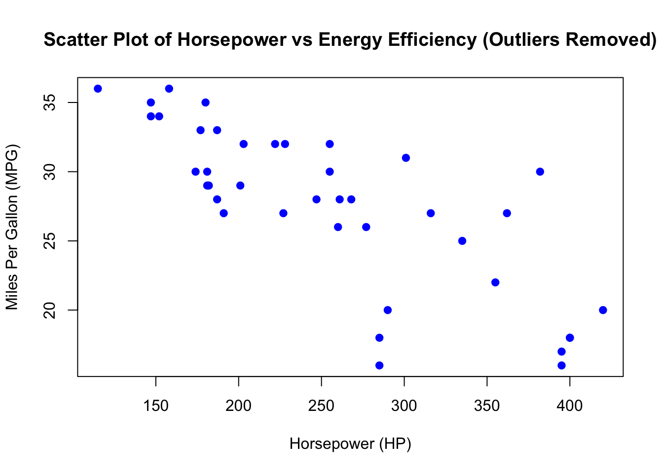
6.6.6 Evaluating Linearity
With the outliers removed, the scatter plot provides a clearer view of the relationship between horsepower and energy efficiency (MPG). Visually, the points appear to gave a linear relationship, though we can see a pattern called heteroscedasticity. We will discuss heteroscedasticity in a latter chapter, so for now the linearity assumption is met.
In the next section, we will proceed to fit a linear regression model to confirm whether the relationship is linear and evaluate the strength of this relationship.
6.7 Simple Linear Regression Model
We will now fit a simple linear regression model to predict energy efficiency (MPG) using horsepower as the predictor. This analysis will help us understand the relationship between these two variables and quantify the impact of horsepower on a vehicle’s fuel efficiency.
Call:
lm(formula = `Energy Efficiency (MPG)` ~ Horsepower, data = car_data_clean)

Residuals:
   Min     1Q Median     3Q    Max
-9.968 -1.966  0.683  1.933  9.241

Coefficients:
             Estimate Std. Error t value Pr(>|t|)
(Intercept) 41.270812   1.864643  22.133  < 2e-16 ***
Horsepower  -0.053695   0.006956  -7.719 2.68e-09 ***
---
Signif. codes:  0 '***' 0.001 '**' 0.01 '*' 0.05 '.' 0.1 ' ' 1

Residual standard error: 3.689 on 38 degrees of freedom
Multiple R-squared:  0.6106,    Adjusted R-squared:  0.6003
F-statistic: 59.58 on 1 and 38 DF, p-value: 2.677e-09The next step is to generate and display the regression equation that quantifies the relationship between horsepower and energy efficiency (MPG).
The estimated regression equation is: \[\hat{MPG} = 41.271 - 0.054 \cdot Horsepower\]
6.8 Model Diagnostics: Residual Analysis
After fitting the simple linear regression model, it is important to check whether the assumptions of linear regression hold. We begin by analyzing the residuals to ensure that the model is well-suited to the data.
A residual plot can help us determine if the residuals (the differences between observed and predicted values) are randomly distributed. Ideally, the residuals should scatter randomly around zero, indicating that the model’s predictions do not systematically deviate from the observed data. We can plot the residuals from the model and add a horizontal line at zero for reference:
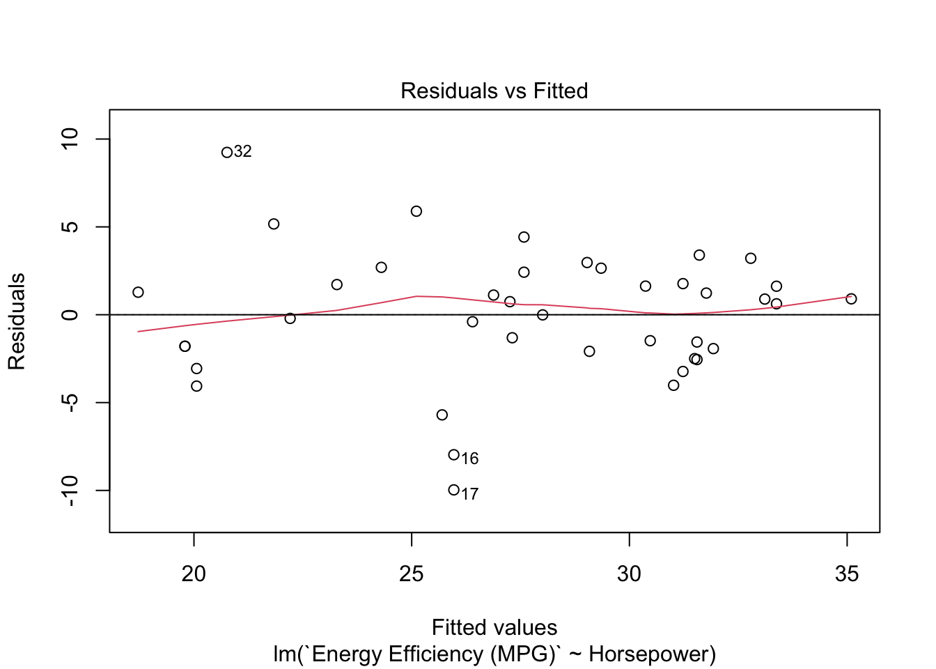
The residual plot generated from the code shows how well the model captures the linear relationship between horsepower and energy efficiency (MPG). A well-fitting model would display no clear pattern or trend in the residuals, meaning they scatter randomly around zero. If the residuals exhibit a clear pattern (e.g., a curve or funnel shape), it may indicate problems with the model, such as non-linearity or heteroscedasticity.
Next, we check if the residuals follow a normal distribution. One of the assumptions of linear regression is that the residuals should be normally distributed. To evaluate this, we plot a histogram of the residuals:
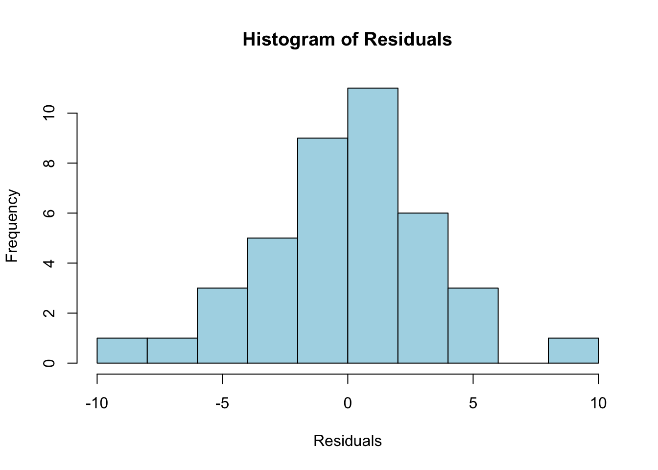
The histogram of residuals provides a visual check for normality. If the residuals are normally distributed, the histogram should form a bell-shaped curve. This would indicate that the residuals are symmetrically distributed around zero, which is important for ensuring valid statistical inferences from the model.
In summary, the residual plot should show random scatter around zero, suggesting that the model adequately captures the relationship between horsepower and energy efficiency without systematic bias. The histogram of residuals should approximate a bell-shaped curve, confirming the assumption of normality. If either of these diagnostics shows issues (e.g., patterns in the residuals or non-normality), further steps might be necessary, such as transforming the variables or considering a different model structure.
6.9 Conclusion
In this analysis, we modeled the relationship between horsepower and energy efficiency (MPG) using a simple linear regression. The results indicate a clear negative relationship between the two variables: as horsepower increases, energy efficiency decreases.
6.9.1 Key Findings:
-
Relationship:
- The negative coefficient of horsepower (-0.0537) suggests that for each additional unit of horsepower, energy efficiency (MPG) decreases by approximately 0.054 miles per gallon, holding all else constant.
- The p-value for the horsepower coefficient (2.68e-09) is highly significant, indicating a strong statistical relationship between horsepower and energy efficiency.
- The R-squared value of 0.6106 suggests that approximately 61.06% of the variability in energy efficiency (MPG) is explained by horsepower, which indicates a moderate fit for a simple linear regression model.
6.9.2 Addressing Outliers:
- Outliers were identified and removed, which improved the accuracy and interpretability of the model.
- The residual diagnostics suggest that the model captures much of the linear relationship, but some deviations and outliers remain, particularly among high-efficiency vehicles (e.g., electric or hybrid vehicles such as the Tesla Model 3).
6.9.3 Next Steps:
- Non-linear Models: Explore whether non-linear models (e.g., quadratic regression or polynomial models) might better capture the relationship between horsepower and energy efficiency, particularly for high-performance or electric vehicles.
- Outlier Analysis: Investigate the characteristics of the outliers to understand if they represent unique types of vehicles, such as electric or hybrid models, that behave differently from traditional gasoline vehicles.
- Refining the Model: Address issues revealed through residual analysis, including potential transformations of variables or alternative models, to improve fit and residual behavior.
6.10 Summary of Packages and Functions Used
In this case study, we used several R packages and functions for data manipulation, model fitting, and diagnostic checking. Below is a summary of the packages, functions, the key arguments used, and links to the R documentation for each function.
6.10.1 Packages Used
-
readxl: Used to read Excel files into R. Key function:read_excel(), which reads data from an Excel file. -
psych: Provides tools for descriptive statistics. Key function:describe(), which generates descriptive statistics for the variables.
6.10.2 Key Functions Used
read_excel("data/car_price.xlsx"): This function reads the dataset from an Excel file into a data frame in R. The key argument is the path to the Excel file, "data/car_price.xlsx", which specifies where the data file is located.
na.omit(): This function removes rows with missing values from the dataset. The argument passed is the data frame, ensuring that any rows containing NA values are excluded from further analysis.
plot(): This function is used to create scatter plots for visualizing relationships between variables. The main arguments include x for the independent variable (e.g., horsepower), y for the dependent variable (e.g., energy efficiency (MPG)), main for the title of the plot, xlab and ylab for axis labels, pch to specify the plotting symbol (e.g., 19 for filled circles), and col to define the color of the points (e.g., "blue").
IQR(): This function calculates the interquartile range (IQR) of a numeric variable. The argument is a numeric vector (e.g., Energy Efficiency (MPG)), and the function returns the difference between the 75th percentile (Q3) and the 25th percentile (Q1).
quantile(): This function computes quantiles of a numeric variable, which are used to determine thresholds for identifying outliers. The arguments include x for the numeric vector and probs for specifying the probability at which to calculate the quantiles (e.g., 0.25 for Q1 and 0.75 for Q3).
points(): This function adds additional points (e.g., outliers) to an existing scatter plot. The key arguments are x for the x-coordinates (e.g., horsepower of outliers), y for the y-coordinates (e.g., energy efficiency (MPG) of outliers), col to specify the color of the points (e.g., "red"), and pch to set the plotting symbol (e.g., 19 for filled circles).
lm(): This function fits a linear regression model. The main arguments are formula, which specifies the relationship to model (e.g., Energy Efficiency (MPG) ~ Horsepower), and data, which defines the data frame containing the variables.
summary(): This function provides a detailed summary of a fitted regression model, including coefficients, R-squared values, and p-values. The argument passed is the fitted model object (e.g., model).
coef(): This function extracts the estimated coefficients (intercept and slope) from a fitted model. The argument is the fitted model object (e.g., model), and it returns the intercept and slope as numeric values.
residuals(): This function extracts the residuals from a fitted linear regression model, which are the differences between the observed and predicted values. The argument is the fitted model object (e.g., model).
plot(model, which = 1): This function creates a residual plot to assess the distribution of residuals and check for potential violations of the linear regression assumptions. The key arguments are model, which specifies the fitted model object, and which = 1, which generates the residuals vs. fitted values plot.
abline(): This function adds a reference line to a plot. The main arguments are h = 0, which adds a horizontal line at zero (useful for residual plots), and col, which specifies the color of the line (e.g., "red").
hist(): This function creates a histogram of the residuals to check for normality. The key arguments are x for the residuals, main for the plot title, xlab for labeling the x-axis, col for specifying the color of the bars (e.g., "lightblue"), and breaks for determining the number of bins in the histogram (e.g., 10).
6.11 Lecture Notes
| Lecture 1: Introduction to Simple Linear Regression | html | |
| Lecture 2: Exploratory Data Analysis (EDA) | html | |
| Lecture 3: Fitting the Simple Linear Regression Model | html | |
| Lecture 4: Residual Diagnostics - Evaluating Model Fit | html | |
| Lecture 5: Interpreting the Model Results | html |
6.12 Homework Assignment: Exploring the Relationship Between Engine Efficiency and MSRP
In this homework assignment, you will apply the simple linear regression workflow to explore the relationship between Energy Efficiency (MPG) and MSRP (USD) using the same vehicle dataset. This exercise will guide you through the steps of loading data, performing exploratory data analysis (EDA), fitting a simple linear regression model, and evaluating the model’s assumptions through residual diagnostics.
6.12.1 Objectives:
- Load and clean the dataset.
- Perform exploratory data analysis (EDA) to visualize the relationship between Energy Efficiency (MPG) and MSRP (USD).
- Fit a simple linear regression model to analyze the relationship.
- Perform residual diagnostics to assess the model’s assumptions.
- Interpret the model results and discuss your findings.
6.12.2 Instructions:
1. Load the Dataset
Use the following code chunk to load the required package and dataset directly from the web:
# Install the openxlsx package if not installed
if (!require(openxlsx)) install.packages("openxlsx")
library(openxlsx)

# Read the Excel file directly from the URL
car_data <- read.xlsx(
  "https://ljkelly3141.github.io/real-world-statistics-with-r/data/car_price.xlsx",
  check.names = FALSE,
  sep.names = " "
)

# View the first few rows of the dataset
head(car_data)After loading the data, inspect the first few rows of the dataset to understand its structure and ensure it was loaded correctly.
2. Exploratory Data Analysis (EDA)
Before fitting a model, perform some initial exploratory data analysis to visualize the relationship between Energy Efficiency (MPG) and MSRP (USD).
- Create a scatter plot to visualize the relationship between the two variables.
- Observe the scatter plot. Does there appear to be a linear relationship between Energy Efficiency (MPG) and MSRP (USD)?
3. Fit a Simple Linear Regression Model
Fit a simple linear regression model where Energy Efficiency (MPG) is the predictor and MSRP (USD) is the response variable.
- Interpret the output from the regression model.
- What does the coefficient of Energy Efficiency (MPG) tell you about the relationship between energy efficiency and MSRP?
- Is the relationship statistically significant? Use the p-values and R-squared values to support your answer.
4. Model Diagnostics: Residual Analysis
Perform residual analysis to evaluate whether the linear regression model meets its assumptions.
- Plot the residuals to check for randomness.
- Plot a histogram of the residuals to check for normality.
- Are the residuals randomly scattered around zero in the residual plot? Does the histogram of residuals indicate that they are normally distributed?
5. Discussion and Interpretation
In your final analysis, address the following questions: - Based on the model output, does Energy Efficiency (MPG) have a significant effect on MSRP (USD)? - What can you conclude about the relationship between engine efficiency and vehicle price? - Do the residual plots suggest any issues with the model’s assumptions (e.g., linearity, homoscedasticity, normality)? - Suggest any further steps you could take if model assumptions are violated (e.g., transformations, using a different model).
6.12.3 Submission Instructions
Please follow these detailed instructions for completing and submitting your assignment. This assignment is to be conducted within the class assignment workspace provided to you. You will create an R Quarto document, incorporating code and analysis as demonstrated in the provided examples. Follow the structure provided in the example code and explanations to guide your analysis. Each required step should correspond to a separate section within your R Quarto document. Utilize the headings feature in Quarto to organize your document (# for main sections, ## for subsections).
Once you have completed the analysis and are satisfied with your document, compile it into an MS Word document and submit it as instructed.