Lecture 4: Residual Diagnostics - Evaluating the Model Fit

Introduction to Residual Analysis

• Objective:
  • The goal of this lecture is to evaluate the model fit using residual diagnostics. This ensures that the assumptions of linear regression hold and helps identify any potential issues such as non-linearity, heteroscedasticity, or outliers that may affect the model.
• Why This Is Important:
  • Residuals are the differences between the observed and predicted values. Analyzing residuals is essential in assessing whether the linear regression model is appropriate and whether it meets key assumptions, including linearity and constant variance (homoscedasticity).
• Key Learning Outcomes:
  • By the end of this lecture, students will be able to:
    • Understand what residuals are and why they are important in regression analysis.
    • Generate residual plots in R.
    • Evaluate residual plots to check for linearity and homoscedasticity.
    • Identify potential issues in the model, such as non-linearity or outliers.

Understanding Residuals

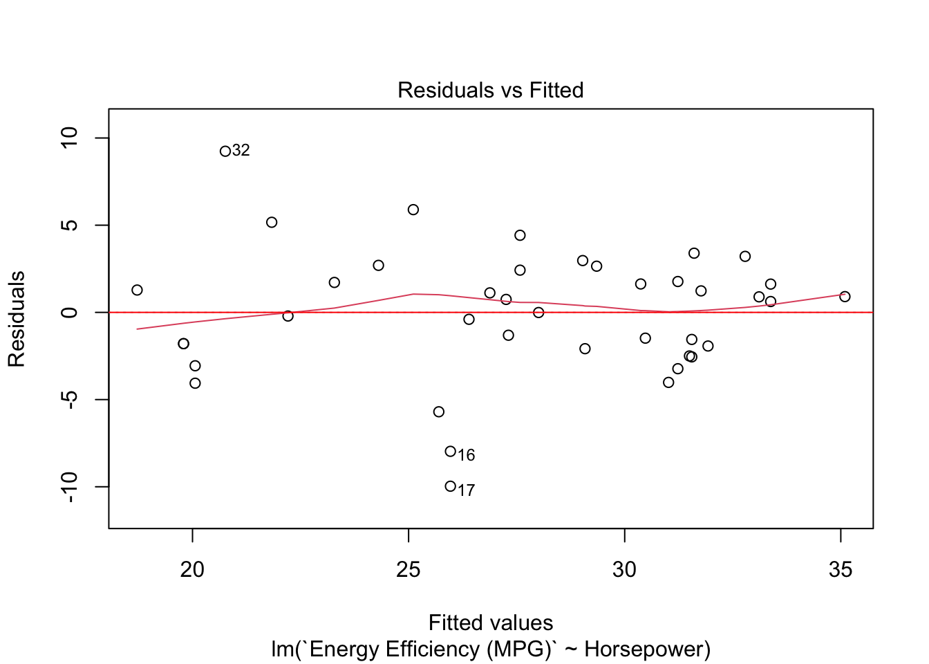
• What Are Residuals?

  • Residuals are the differences between the actual observed values of the response variable (in this case, Energy Efficiency (MPG)) and the values predicted by the linear regression model.

  \[ \text{Residual} = \text{Observed} - \text{Predicted} \]

  • The goal is for residuals to be randomly distributed around zero, which would indicate that the model captures the underlying relationship well.

• Why Analyze Residuals?

  • Linearity: Residuals should show no patterns. If patterns exist, it may indicate a non-linear relationship between Horsepower and MPG.
  • Homoscedasticity: The spread of residuals should be roughly the same across all levels of the predictor (i.e., Horsepower). If the variance of residuals changes (heteroscedasticity), the model may not be valid.
  • Normality of Residuals: Residuals should follow a normal distribution for valid statistical inferences.

Generating Residual Plots in R

Code Chunk: Plotting Residuals

# Plot residuals vs. fitted values
plot(model, which = 1)
abline(h = 0, col = "red")

Breaking Down the Code

• plot(model, which = 1): This creates a residual plot, plotting residuals against the fitted (predicted) values. The residuals should scatter randomly around zero for a well-fitted model.
• abline(h = 0, col = "red"): Adds a horizontal red line at zero to visually emphasize the center point, helping assess whether residuals are evenly distributed around zero.

Interpreting the Residual Plot

• Random Scatter: If the residuals appear to be randomly scattered around zero, it suggests that the linearity assumption holds. If there is a clear pattern (e.g., a curve or a funnel shape), this indicates potential problems such as non-linearity or heteroscedasticity.
• Potential Issues:
  • Non-linearity: A curved pattern in the residuals indicates that the relationship between Horsepower and MPG might not be linear.
  • Homoscedasticity: If the spread of residuals widens or narrows as Horsepower increases, this indicates heteroscedasticity, which violates the assumption of constant variance.

Checking for Normality of Residuals

Code Chunk: Plotting a Histogram of Residuals

# Plot a histogram of residuals
hist(residuals(model), 
     main = "Histogram of Residuals", 
     xlab = "Residuals", 
     col = "lightblue", 
     breaks = 10)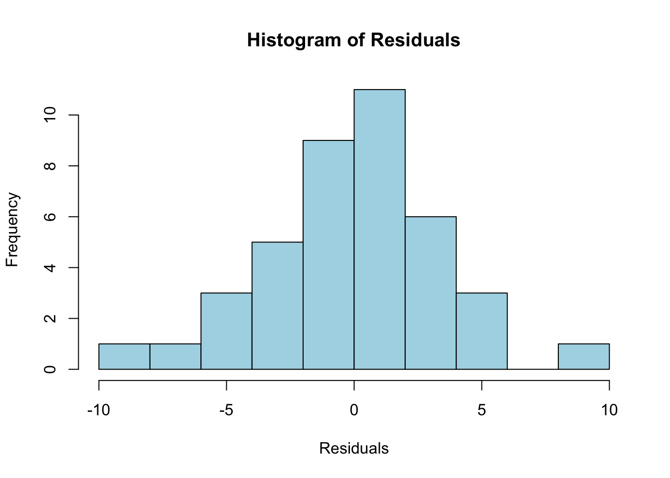

Breaking Down the Code

• hist(residuals(model)): This command creates a histogram of the residuals to check for normality. If the residuals are normally distributed, the histogram should show a bell-shaped curve.
• breaks = 10: Specifies the number of bins in the histogram for better visualization.
• col = "lightblue": Adds a color to the bars for better visibility.

Interpreting the Histogram

• Normal Distribution: Ideally, the residuals should form a roughly bell-shaped curve, indicating that the residuals follow a normal distribution.
• Signs of Non-Normality: If the histogram is skewed or has heavy tails, this suggests that the residuals are not normally distributed, which may affect the validity of hypothesis tests in the regression model.

Additional Diagnostic Plot: Q-Q Plot for Residuals

Code Chunk: Generating a Q-Q Plot

# Q-Q plot for residuals
qqnorm(residuals(model))
qqline(residuals(model), col = "red")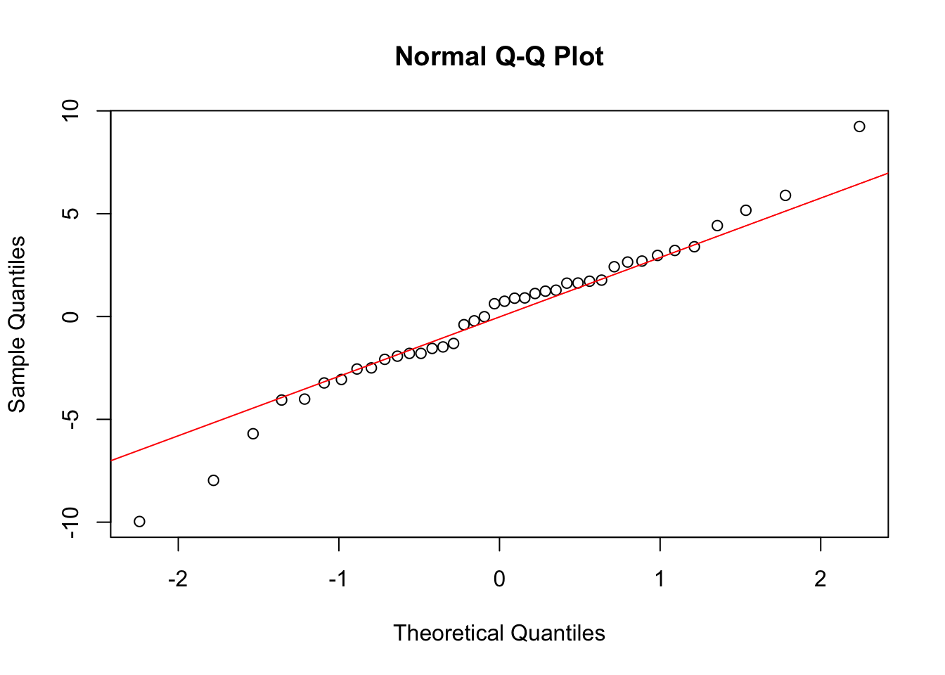

Breaking Down the Code

• qqnorm(): Creates a Q-Q plot that compares the residuals to a normal distribution. If the residuals follow a normal distribution, they should fall along a straight line.
• qqline(): Adds a reference line to the Q-Q plot to help visualize how well the residuals match the expected normal distribution.

Interpreting the Q-Q Plot

• Straight Line: If the points closely follow the red line, it suggests that the residuals are normally distributed.
• Deviations from Line: Significant deviations from the line, especially at the tails, indicate non-normality. If the residuals fall above or below the line, it may suggest skewness or heavy tails in the data.

Summary of Residual Diagnostics

• Residual Plot: Should show a random scatter of points around zero. Patterns in the residuals suggest non-linearity or heteroscedasticity.
• Histogram of Residuals: Should display a bell-shaped curve, indicating that the residuals follow a normal distribution.
• Q-Q Plot: Helps confirm whether the residuals are normally distributed. Deviations from the straight line indicate non-normality.

Conclusion and Next Steps

• Summary:
  • In this lecture, we performed residual diagnostics to assess the assumptions of the linear regression model.
  • We examined the residual plot to check for linearity and homoscedasticity, and used a histogram and Q-Q plot to check for normality of residuals.
• Next Steps:
  • If the residual diagnostics reveal any issues, the next step would be to consider alternative models (e.g., non-linear regression) or apply transformations to the data.
  • In the next lecture, we will focus on refining the model and discussing strategies for handling outliers and improving the fit of the model.

Assignment for Students:

1. Generate a residual plot for your regression model and assess whether the residuals are randomly distributed around zero.
2. Create a histogram and Q-Q plot of the residuals and evaluate whether they follow a normal distribution.
3. Submit a brief summary of your findings, including whether you identified any issues with the model’s assumptions.

This lecture guides students through the residual diagnostics process, emphasizing the importance of evaluating the model’s assumptions before drawing conclusions.