9 Dealing with Categorical Data

Categorical data is a fundamental aspect of business analytics, representing information that can be divided into distinct categories or groups. Whether it’s classifying products into different types, segmenting customers based on demographics, or analyzing employee roles, categorical data is omnipresent in business contexts. Understanding how to preprocess, analyze, and model categorical data is crucial for making informed decisions and gaining insights from data. This chapter will explore the various techniques for handling categorical data, from basic concepts to advanced methods, and demonstrate their practical applications using R.

9.1 Chapter Goals

Upon concluding this chapter, readers will be equipped with the skills to:

Understand the different types of categorical data (nominal and ordinal) and their significance in business analytics.
Preprocess categorical data by handling missing values, addressing outliers, and applying appropriate encoding techniques.
Analyze datasets containing only categorical data using cross-tabulations and chi-square tests.
Perform ANOVA to compare means across different groups in datasets with mixed categorical and continuous variables.
Incorporate categorical variables into linear regression models using dummy variables and interpret their coefficients.
Address multicollinearity in regression models with categorical variables.
Apply advanced techniques such as feature hashing, embeddings, decision trees, random forests, and gradient boosting machines to handle high cardinality and complex categorical data.
Use logistic regression to model categorical dependent variables and interpret the results.

9.2 Introduction to Categorical Data

Categorical data refers to variables that classify observations into distinct groups or categories based on qualitative attributes. Unlike numerical data, which quantifies measurements, categorical data focuses on classifying data points into categories. These categories can be either nominal or ordinal. Nominal variables represent categories that do not have a specific order or ranking, such as product types, payment methods, or customer segments. The key characteristic of nominal data is that the categories are merely labels without any inherent order. On the other hand, ordinal variables are categorical variables that have a defined order or ranking, but the intervals between the categories are not necessarily equal. Examples of ordinal data include customer satisfaction ratings, such as poor, fair, good, excellent, or education levels like high school, bachelor’s degree, and master’s degree.

In business analytics, categorical data is essential for understanding and analyzing qualitative aspects of data. For instance, it allows for the classification of customers into distinct segments based on behavior, preferences, or demographics. It also helps in organizing products into categories like electronics, clothing, and groceries, which is important for inventory management and marketing strategies. Additionally, categorical data is useful for differentiating between various job roles or departments within an organization, aiding in the analysis of performance, satisfaction, or turnover rates. Categorical data thus provides the foundation for businesses to make sense of qualitative attributes, which are crucial for informed decision-making and strategic planning.

In R, categorical data is often represented as factor variables. A factor variable stores categorical data along with its corresponding levels, making it easier to work with in statistical modeling and analysis. Factors are particularly important in R because they ensure that categorical data is treated appropriately in various statistical functions and models. To work with categorical data in R, a vector can be converted into a factor using the as.factor() function. This conversion tells R to treat the data as categorical rather than numerical. For example, consider a vector of numerical values representing different product categories. By converting this vector into a factor, R is instructed to treat these values as categories rather than numbers. Factor variables are critical for the correct interpretation of categorical data in statistical models, such as regression analysis. Without converting categorical data into factors, R might treat the data as continuous, leading to incorrect analysis and interpretation. Understanding how to handle categorical data in R is vital for conducting accurate and meaningful analyses, especially in business contexts where such data is prevalent.

9.3 Types of Categorical Variables and Factor Variables in R

Categorical variables can be classified into two main types: nominal and ordinal variables. Each type has distinct characteristics that influence how the data is analyzed and interpreted.

Nominal Variables are categorical variables that do not have any intrinsic order or ranking among the categories. The categories are mutually exclusive, meaning that each observation can belong to only one category at a time. Importantly, there is no inherent ranking or order among these categories, and they are treated as labels rather than values that can be compared. Examples of nominal variables include:

Vehicle Types: Sedan, SUV, Truck, Motorcycle.
Job Roles: Engineer, Manager, Analyst, Technician.
Example from Built-in Dataset: In the iris dataset in R, the Species variable is a nominal variable, with categories such as setosa, versicolor, and virginica.

Ordinal Variables, on the other hand, are categorical variables that have a defined order or ranking. The key characteristic of ordinal variables is that the categories can be arranged in a meaningful sequence, but the intervals between these categories are not necessarily equal. This means that while you can rank the categories, the difference between them is not uniform or consistent. Examples of ordinal variables include:

Spiciness Levels in Food: Mild, Medium, Hot, Extra hot.
Performance Ratings: Needs improvement, Meets expectations, Exceeds expectations, Outstanding.
Example from Built-in Dataset: In the mtcars dataset in R, the gear variable could be considered ordinal if you assume a natural progression in the number of gears (3, 4, 5 gears), even though the exact intervals between them are not uniform.

Understanding the distinction between nominal and ordinal variables is essential for proper data analysis, as the type of categorical variable determines the appropriate statistical methods and interpretations. Using examples from built-in datasets like iris and mtcars in R helps illustrate these concepts in a practical context.

To work with categorical data in R, you can convert a vector into a factor using the as.factor() function. This conversion tells R to treat the data as categorical rather than numerical. For example, consider a numerical variable that represents different product categories:

product_categories <- c(1, 2, 1, 3, 2)
product_categories_factor <- as.factor(product_categories)

In this example, the product_categories vector contains numerical values, which could represent different product types. By converting this vector into a factor using as.factor(), you instruct R to treat these values as categories rather than numbers. Once converted to a factor, the data is recognized as categorical, and R will handle it accordingly in subsequent analyses.

R provides several built-in datasets where categorical data is stored as factors. For instance, in the iris dataset, the Species variable is a factor, representing the three species of iris flowers: setosa, versicolor, and virginica. The Species variable is already a factor when you load the dataset, making it easy to analyze the categorical nature of this variable in statistical models:

data(iris)
str(iris$Species)

 Factor w/ 3 levels "setosa","versicolor",..: 1 1 1 1 1 1 1 1 1 1 ...

Another example can be found in the mtcars dataset. While the gear variable in mtcars is stored as a numerical variable, it can be converted into a factor if you want to treat the number of gears as a categorical variable in your analysis:

data(mtcars)
mtcars$gear_factor <- as.factor(mtcars$gear)
str(mtcars$gear_factor)

 Factor w/ 3 levels "3","4","5": 2 2 2 1 1 1 1 2 2 2 ...

In this example, the gear variable, which represents the number of gears in the cars, is converted into a factor. This allows you to analyze the variable as a categorical one, distinguishing between cars with 3, 4, or 5 gears without assuming a numerical relationship between them.

Factor variables are essential for the correct interpretation of categorical data in statistical models, such as regression analysis. In these models, R needs to distinguish between categorical and numerical data to apply the appropriate techniques and generate meaningful results. For instance, in a regression model, if categorical variables are not properly converted to factors, R might treat them as continuous variables. This could lead to incorrect analysis and misinterpretation of the results, as the statistical methods applied would not account for the categorical nature of the data.

By converting categorical data into factor variables, you ensure that R applies the correct methods, leading to accurate and reliable results. This practice is particularly important in business analytics, where categorical data is often prevalent, and the correct interpretation of such data can significantly impact decision-making and strategic planning. Understanding how to handle categorical data in R through factor variables sets the foundation for conducting robust statistical analyses in various contexts.

9.4 Preprocessing Categorical Data

Preprocessing categorical data is a critical step in ensuring that your data is ready for analysis. This involves identifying and addressing outliers, encoding categorical variables into formats that can be used effectively in statistical models, and reordering factor levels to reflect meaningful orderings in your analysis.

Identifying and Addressing Outliers in Categorical Data

Outliers in categorical data refer to categories that appear infrequently or that deviate significantly from the rest of the dataset. Identifying and addressing these outliers can help improve the quality of the analysis:

Frequency-based Detection: One way to detect outliers in categorical data is by examining the frequency of each category. Categories that occur very infrequently might be considered outliers.

# Example: Detecting outliers by frequency
table(iris$Species)


    setosa versicolor  virginica 
        50         50         50

Combining Rare Categories: Once outliers are identified, one common

approach is to combine them into a single “Other” category, reducing their impact on the analysis.

# Example: Combining rare categories
library(dplyr)


Attaching package: 'dplyr'

The following objects are masked from 'package:stats':

    filter, lag

The following objects are masked from 'package:base':

    intersect, setdiff, setequal, union

iris <- iris %>%
  mutate(Species = if_else(Species == "Unknown", "Other", Species))

Encoding Categorical Variables

Encoding categorical variables is essential for transforming them into a format that can be utilized in statistical models, particularly those that require numerical input. There are several encoding techniques available:

One-Hot Encoding: This technique creates a binary column for each category in the variable. One-hot encoding is particularly useful when there is no ordinal relationship between categories. However, it can lead to a significant increase in the number of columns, especially with variables that have many categories.

# Example: One-hot encoding using ifelse() and mutate()
iris <- iris %>%
  mutate(Species_setosa = if_else(Species == "setosa", 1, 0),
         Species_versicolor = if_else(Species == "versicolor", 1, 0),
         Species_virginica = if_else(Species == "virginica", 1, 0))

In this example, each species in the Species variable is transformed into a separate binary column: setosa, versicolor, and virginica are represented by their own binary indicators. This method is useful when dealing with nominal variables that have no inherent order.

Label Encoding: In label encoding, each category is assigned a unique integer. This method is simple and effective for ordinal variables where there is a meaningful order between categories. However, it may introduce unintended ordinal relationships if used with nominal variables.

# Example: Label encoding a categorical variable
iris <- iris %>%
  mutate(Species_label = as.numeric(Species))

Warning: There was 1 warning in `mutate()`.
ℹ In argument: `Species_label = as.numeric(Species)`.
Caused by warning:
! NAs introduced by coercion

Binary Encoding: Binary encoding is a hybrid approach that combines the simplicity of label encoding with the dimensionality reduction of one-hot encoding. You can implement binary encoding in R using a case_when() statement from the dplyr package.

# Example: Binary encoding using case_when() statement from dplyr
iris <- iris %>%
  mutate(Species_binary = case_when(
    Species == "setosa" ~ "01",
    Species == "versicolor" ~ "10",
    Species == "virginica" ~ "11",
    TRUE ~ NA_character_
  ))

In this example, the Species variable in the iris dataset is encoded into binary strings. Each species is assigned a unique binary code: setosa becomes “01,” versicolor becomes “10,” and virginica becomes “11.” The TRUE ~ NA_character_ part ensures that any unexpected values are handled by assigning NA. This method is straightforward and provides a clear, readable alternative to nested ifelse() statements.

Reordering Factor Levels

Reordering factor levels is an important preprocessing step when working with categorical data, particularly when the order of categories carries meaning or when you want to control the order in which categories appear in visualizations and analyses. By default, R orders factor levels alphabetically, but this might not reflect the logical or meaningful order you need.

You can reorder factor levels in R using the fct_relevel() function from the forcats package, which allows you to specify the desired order of levels explicitly:

# Example: Reordering factor levels using fct_relevel() from the forcats package
library(forcats)

iris <- iris %>%
  mutate(Species = fct_relevel(Species, "virginica", "versicolor", "setosa"))

In this example, the Species factor is reordered so that virginica appears first, followed by versicolor, and then setosa. Reordering factor levels can be particularly useful when creating plots or when performing analyses where the order of categories has significance, such as in ordinal regression or when controlling the sequence of categories in bar plots.

Reordering factors ensures that your categorical data is presented and analyzed in a way that aligns with your research goals or business requirements, leading to more meaningful and interpretable results.

Choosing the Right Encoding Method

Selecting the appropriate encoding method depends on the specific characteristics of the dataset and the requirements of the analysis:

One-Hot Encoding is ideal for nominal variables without a natural order but may lead to high dimensionality in large datasets.
Label Encoding is suitable for ordinal variables where the order of categories is meaningful, but it can introduce biases if applied to nominal variables.
Binary Encoding offers a compromise between dimensionality and simplicity, reducing the number of columns while retaining information, making it useful when dealing with high-cardinality categorical variables.

By carefully considering the nature of the categorical data and the goals of your analysis, you can select the most appropriate preprocessing techniques to ensure your data is ready for accurate and effective modeling. Reordering factor levels and selecting the correct encoding method are crucial steps that can significantly impact the quality and interpretability of your statistical analyses.

9.5 Analyzing Datasets with Only Categorical Data

When working with datasets that contain only categorical data, it is essential to use appropriate techniques to analyze the relationships and patterns within the data. Two fundamental methods for analyzing categorical data are cross-tabulation and Chi-Square tests. These methods help in understanding the associations between categorical variables and in testing hypotheses about their distributions.

Cross Tabulation

Cross tabulation, also known as a contingency table, is a method for analyzing the relationship between two or more categorical variables by displaying their frequency distribution in a matrix format. This approach allows you to see how different categories interact with one another, helping to identify patterns and relationships within the data. The primary purpose of cross tabulation is to understand relationships between categorical variables, uncovering patterns and associations that may not be immediately apparent when looking at raw data.

To implement cross tabulation in R, you can start by using the mtcars dataset. Begin by converting the cyl (number of cylinders) and am (transmission type) variables into factors to treat them as categorical variables:

data(mtcars)
mtcars$cyl <- as.factor(mtcars$cyl)
mtcars$am <- as.factor(mtcars$am)

Next, use the table() function to create a cross tabulation of cyl and am:

cross_tab <- table(mtcars$cyl, mtcars$am)

This cross tabulation can be displayed to examine the relationship between the number of cylinders and transmission type:

print(cross_tab)

Optionally, you can add more readable labels to the table for better interpretation:

colnames(cross_tab) <- c("Automatic", "Manual")
rownames(cross_tab) <- c("4 Cylinders", "6 Cylinders", "8 Cylinders")
print(cross_tab)

             
              Automatic Manual
  4 Cylinders         3      8
  6 Cylinders         4      3
  8 Cylinders        12      2

After creating the cross tabulation, further analysis can be conducted by generating proportion tables or performing Chi-Square tests to evaluate the statistical significance of the observed relationships.

Chi-Square Tests

Chi-Square tests are commonly used to analyze categorical data, specifically to test hypotheses about the distribution of categorical variables and their independence from one another. The Chi-Square Test of Goodness of Fit and the Chi-Square Test of Independence are two key types of Chi-Square tests.

The Chi-Square Test of Goodness of Fit is used to determine whether the observed frequencies of a single categorical variable match the expected frequencies based on a hypothesized distribution. This test helps assess whether a categorical variable follows a specific distribution pattern. The test statistic for the Chi-Square Test of Goodness of Fit is calculated using the formula:

\[ \chi^2 = \sum \frac{(O_i - E_i)^2}{E_i} \]

where \(O_i\) represents the observed frequency for category \(i\) and \(E_i\) represents the expected frequency for category \(i\). This formula calculates the sum of the squared differences between the observed and expected frequencies, divided by the expected frequencies for each category.

To perform this test in R, you might create observed data representing car colors:

observed_colors <- c(50, 30, 20)  # Example: Red, Blue, Green cars

Assume an equal distribution of car colors for the expected proportions:

expected_proportions <- c(1/3, 1/3, 1/3)  # Assuming equal proportions

You can then perform the Chi-Square Test of Goodness of Fit using the chisq.test() function:

chisq_test_gof <- chisq.test(x = observed_colors, p = expected_proportions)
print(chisq_test_gof)


    Chi-squared test for given probabilities

data:  observed_colors
X-squared = 14, df = 2, p-value = 0.0009119

The test output includes the Chi-Square statistic, degrees of freedom, and p-value. The p-value is particularly important as it helps determine whether the observed distribution significantly differs from the expected distribution.

The Chi-Square Test of Independence tests whether there is a significant association between two categorical variables, helping to determine whether the presence or absence of one variable is related to the presence or absence of another. The formula for the Chi-Square Test of Independence is similar to that of the Goodness of Fit test:

\[ \chi^2 = \sum \frac{(O_{ij} - E_{ij})^2}{E_{ij}} \]

where \(O_{ij}\) represents the observed frequency in the cell corresponding to row \(i\) and column \(j\), and \(E_{ij}\) represents the expected frequency for that cell. The expected frequency \(E_{ij}\) is calculated as:

\[ E_{ij} = \frac{(Row_i \times Col_j)}{Total} \]

where \(Row_i\) is the total frequency for row \(i\), \(Col_j\) is the total frequency for column \(j\), and \(Total\) is the overall total number of observations.

For example, to assess the independence between the type of transmission and the number of cylinders in the mtcars dataset, you would first create a cross tabulation of cyl and am as described earlier. Then, perform the Chi-Square Test of Independence using the chisq.test() function:

chisq_test_indep <- chisq.test(cross_tab)

Warning in chisq.test(cross_tab): Chi-squared approximation may be incorrect

print(chisq_test_indep)


    Pearson's Chi-squared test

data:  cross_tab
X-squared = 8.7407, df = 2, p-value = 0.01265

The results include the Chi-Square statistic, degrees of freedom, and p-value. A low p-value suggests a significant association between the two variables, indicating they are not independent.

These methods form the foundation for analyzing categorical data, enabling you to uncover relationships and test hypotheses in datasets consisting entirely of categorical variables. By using cross tabulation and Chi-Square tests, you can gain valuable insights into the structure and associations within your categorical data.

9.6 Analyzing Datasets with Mixed Data Types (Categorical and Continuous)

When working with datasets that contain both categorical and continuous variables, it’s essential to apply appropriate statistical methods to analyze the relationships between these different types of data. One such method is Analysis of Variance (ANOVA), which is widely used to compare the means of a continuous variable across different levels of a categorical variable. However, when the assumptions of ANOVA are violated, alternative methods like the Kruskal-Wallis test or Welch’s ANOVA may be more appropriate.

ANOVA (Analysis of Variance)

ANOVA, or Analysis of Variance, is a statistical method used to compare the means of a continuous variable across different levels of a categorical variable. The fundamental principle of ANOVA is to assess whether the variation between the group means is greater than the variation within the groups. When the variation between groups is significantly larger, it suggests that the group means are not all equal, indicating a statistically significant difference among the groups.

ANOVA is particularly valuable when comparing the means across multiple groups to determine if at least one group mean differs from the others. It is widely employed in experimental designs and business analytics to compare groups such as different customer segments, product categories, or sales regions. For instance, a company might use ANOVA to compare average sales across various regions to determine if there is a significant difference in sales performance by region.

Types of ANOVA

There are several types of ANOVA, each suited to different experimental designs and data structures:

One-Way ANOVA:
One-Way ANOVA compares the means of one continuous dependent variable across multiple levels of a single categorical independent variable. For example, you might use One-Way ANOVA to compare the average sales (continuous) across different product categories (categorical).
Two-Way ANOVA:
Two-Way ANOVA examines the effect of two categorical independent variables on one continuous dependent variable and also considers the interaction between the two categorical variables. For instance, you could analyze how both product category and region affect sales and whether the effect of the product category varies by region.
Repeated Measures ANOVA:
Repeated Measures ANOVA is used when the same subjects are measured under different conditions or at different points in time. An example would be measuring customer satisfaction (continuous) before and after a product update across different customer segments (categorical).

Assumptions of ANOVA

For ANOVA to produce valid results, several key assumptions must be met:

Independence: The observations must be independent of each other. This means that the data collected in one group should not influence the data collected in another group. Independence is usually ensured by proper experimental design or data collection procedures.
Normality: The dependent variable should be approximately normally distributed within each group. This assumption is particularly important when the sample sizes are small. If the data are not normally distributed, the F-test used in ANOVA might not be valid. You can check this assumption using normality tests such as the Shapiro-Wilk test or by visual inspection using Q-Q plots.
Homogeneity of Variances (Homoscedasticity): The variance among the groups should be approximately equal. This assumption ensures that the F-test is valid when comparing group means. If the variances are not equal, the ANOVA results might be misleading. The homogeneity of variances can be tested using Levene’s Test or Bartlett’s Test.

Violations of these assumptions can lead to incorrect conclusions. If the assumptions of ANOVA are not met, you might consider using alternative methods such as the Kruskal-Wallis test or Welch’s ANOVA, which are more robust to these violations.

R Implementation of ANOVA

To perform ANOVA in R, we can use the mtcars dataset, where the dependent variable is continuous (e.g., mpg) and the independent variable is categorical (e.g., cyl for the number of cylinders).

Set Up the Data: Ensure the categorical variable is treated as a factor:

mtcars$cyl <- as.factor(mtcars$cyl)

Perform One-Way ANOVA: Use the aov() function to perform a one-way ANOVA, comparing the mean miles per gallon (mpg) across different cylinder groups (cyl):

anova_result <- aov(mpg ~ cyl, data = mtcars)
summary(anova_result)

            Df Sum Sq Mean Sq F value   Pr(>F)    
cyl          2  824.8   412.4    39.7 4.98e-09 ***
Residuals   29  301.3    10.4                     
---
Signif. codes:  0 '***' 0.001 '**' 0.01 '*' 0.05 '.' 0.1 ' ' 1

Perform Two-Way ANOVA: Extend the ANOVA to include a second factor, such as transmission type (am):

anova_result_two_way <- aov(mpg ~ cyl * am, data = mtcars)
summary(anova_result_two_way)

            Df Sum Sq Mean Sq F value   Pr(>F)    
cyl          2  824.8   412.4  44.852 3.73e-09 ***
am           1   36.8    36.8   3.999   0.0561 .  
cyl:am       2   25.4    12.7   1.383   0.2686    
Residuals   26  239.1     9.2                     
---
Signif. codes:  0 '***' 0.001 '**' 0.01 '*' 0.05 '.' 0.1 ' ' 1

This code examines the effects of both cyl and am on mpg and their interaction.

Check Assumptions:
- Normality: Use diagnostic plots or tests like the Shapiro-Wilk test to assess normality:

shapiro.test(residuals(anova_result))


    Shapiro-Wilk normality test

data:  residuals(anova_result)
W = 0.97065, p-value = 0.5177

Homogeneity of Variances: Use Levene’s Test from the car package to test for equal variances:

library(car)

Loading required package: carData


Attaching package: 'car'

The following object is masked from 'package:dplyr':

    recode

leveneTest(mpg ~ cyl, data = mtcars)

Interpret the Results:
- F-Statistic: The F-statistic indicates the ratio of the variance between the group means to the variance within the groups. A higher F-statistic suggests a greater difference between the groups.
- p-value: If the p-value is less than the significance level (typically 0.05), you reject the null hypothesis, indicating that at least one group mean is significantly different from the others.
- Post-Hoc Tests: If ANOVA indicates significant differences, post-hoc tests like Tukey’s HSD can identify which specific groups differ:

TukeyHSD(anova_result)

  Tukey multiple comparisons of means
    95% family-wise confidence level

Fit: aov(formula = mpg ~ cyl, data = mtcars)

$cyl
          diff        lwr        upr     p adj
6-4  -6.920779 -10.769350 -3.0722086 0.0003424
8-4 -11.563636 -14.770779 -8.3564942 0.0000000
8-6  -4.642857  -8.327583 -0.9581313 0.0112287

This test compares all possible pairs of means to see which ones are significantly different.

Kruskal-Wallis Test

The Kruskal-Wallis test is a non-parametric alternative to One-Way ANOVA, used to compare the medians of a continuous variable across different groups when the assumption of normality is not met.

This test is particularly useful when the data does not meet the assumptions required for ANOVA, as it does not require the data to be normally distributed or the variances to be equal. Instead of using the raw data, the Kruskal-Wallis test is based on the ranks of the data, making it a robust option in cases where ANOVA’s assumptions are violated.

R Implementation:

To perform the Kruskal-Wallis test in R, you can use the kruskal.test() function:

kruskal_result <- kruskal.test(mpg ~ cyl, data = mtcars)
print(kruskal_result)


    Kruskal-Wallis rank sum test

data:  mpg by cyl
Kruskal-Wallis chi-squared = 25.746, df = 2, p-value = 2.566e-06

This test compares the median miles per gallon (mpg) across different cylinder groups (cyl). The test output includes the Kruskal-Wallis statistic and the p-value, which you can use to determine if there are significant differences between the groups.

Welch’s ANOVA

Welch’s ANOVA is an alternative to the traditional One-Way ANOVA that is specifically designed to be more robust when the assumption of homogeneity of variances is violated. It is particularly useful in situations where the variances across groups are unequal.

Welch’s ANOVA is employed when there is a suspicion or knowledge that the assumption of equal variances does not hold. Unlike standard ANOVA, which assumes homogeneity of variances, Welch’s ANOVA adjusts the degrees of freedom when calculating the p-value, making it a more reliable method under conditions of unequal variances.

R Implementation:

To perform Welch’s ANOVA in R, you can use the oneway.test() function with the var.equal = FALSE parameter:

welch_anova_result <- oneway.test(mpg ~ cyl, data = mtcars, var.equal = FALSE)
print(welch_anova_result)


    One-way analysis of means (not assuming equal variances)

data:  mpg and cyl
F = 31.624, num df = 2.000, denom df = 18.032, p-value = 1.271e-06

This test compares the mean miles per gallon (mpg) across different cylinder groups (cyl), taking into account unequal variances across these groups. The output includes the Welch F-statistic, adjusted degrees of freedom, and p-value.

Categorical Data in the Context of Linear Regression

In linear regression models, categorical variables must be transformed into a numerical format before they can be included. This is typically done by creating dummy variables, which are binary (0/1) indicators for each category of the categorical variable. For example, suppose we have a categorical variable for transmission

type (am), where 0 represents automatic and 1 represents manual. In a regression model, this would be included as a dummy variable to compare the effect of transmission type on a continuous outcome, such as miles per gallon (mpg).

To implement this in R, you can create dummy variables using the model.matrix() function:

dummy_vars <- model.matrix(~ am - 1, data = mtcars)

These dummy variables can then be included in a regression model using the lm() function:

model <- lm(mpg ~ am, data = mtcars)
summary(model)


Call:
lm(formula = mpg ~ am, data = mtcars)

Residuals:
    Min      1Q  Median      3Q     Max 
-9.3923 -3.0923 -0.2974  3.2439  9.5077 

Coefficients:
            Estimate Std. Error t value Pr(>|t|)    
(Intercept)   17.147      1.125  15.247 1.13e-15 ***
am1            7.245      1.764   4.106 0.000285 ***
---
Signif. codes:  0 '***' 0.001 '**' 0.01 '*' 0.05 '.' 0.1 ' ' 1

Residual standard error: 4.902 on 30 degrees of freedom
Multiple R-squared:  0.3598,    Adjusted R-squared:  0.3385 
F-statistic: 16.86 on 1 and 30 DF,  p-value: 0.000285

The coefficient for the dummy variable in the regression output indicates the difference in the dependent variable (e.g., mpg) between the reference category (e.g., automatic transmission) and the category represented by the dummy variable (e.g., manual transmission).

Interpretation of Dummy Variable Coefficients

In a linear regression model with dummy variables, the intercept represents the expected value of the dependent variable (e.g., mpg) for the reference category (e.g., automatic transmission). The coefficient for each dummy variable represents the change in the dependent variable relative to the reference category. This can be interpreted as a piecewise-defined function. For a model with a single dummy variable \(D\) (where \(D = 0\) for the reference category and \(D = 1\) for the other category), the regression equation is:

\[ Y = \begin{cases} \beta_0 & \text{if } D = 0 \\ \beta_0 + \beta_1 & \text{if } D = 1 \end{cases} \]

Here, \(\beta_0\) is the intercept (expected value of \(Y\) when \(D = 0\)), and \(\beta_1\) is the coefficient for the dummy variable (the difference in \(Y\) between \(D = 1\) and \(D = 0\)).

Example Interpretation:
Suppose the regression model output is:

\[ mpg = 20 + 5 \cdot \text{am} \]

If \(am = 0\) (automatic transmission), the expected \(mpg\) is 20. If \(am = 1\) (manual transmission), the expected \(mpg\) is 25 (20 + 5), indicating that manual transmission is associated with 5 more miles per gallon compared to automatic transmission.

Interaction Terms

Interaction terms in a regression model allow for the examination of how the relationship between one predictor and the outcome variable might change depending on the level of another predictor. This is particularly useful when the effect of one variable might differ depending on the category of another variable.

Example:
Suppose we want to examine whether the effect of weight (wt) on mpg differs depending on the transmission type (am). The interaction term would be included in the model as:

model_interaction <- lm(mpg ~ wt * am, data = mtcars)
summary(model_interaction)


Call:
lm(formula = mpg ~ wt * am, data = mtcars)

Residuals:
    Min      1Q  Median      3Q     Max 
-3.6004 -1.5446 -0.5325  0.9012  6.0909 

Coefficients:
            Estimate Std. Error t value Pr(>|t|)    
(Intercept)  31.4161     3.0201  10.402 4.00e-11 ***
wt           -3.7859     0.7856  -4.819 4.55e-05 ***
am1          14.8784     4.2640   3.489  0.00162 ** 
wt:am1       -5.2984     1.4447  -3.667  0.00102 ** 
---
Signif. codes:  0 '***' 0.001 '**' 0.01 '*' 0.05 '.' 0.1 ' ' 1

Residual standard error: 2.591 on 28 degrees of freedom
Multiple R-squared:  0.833, Adjusted R-squared:  0.8151 
F-statistic: 46.57 on 3 and 28 DF,  p-value: 5.209e-11

R Implementation:

Create Interaction Terms: Use the * or : operators in lm() to include interaction terms in the model.
Interpret the Results: The coefficient of the interaction term indicates how much the effect of one variable (e.g., wt) on the dependent variable (mpg) changes when moving from one category of the interacting variable (e.g., am) to another.
Piecewise Interpretation: The resulting model can be interpreted as having different slopes for the relationship between wt and mpg depending on the value of am.

Interpreting Interactions

When interaction terms are included in a regression model, the interpretation of the coefficients becomes more nuanced. The coefficient for the main effect of one variable (e.g., wt) now represents the effect of that variable when the interacting variable (e.g., am) is at its reference level. The coefficient of the interaction term itself tells you how much the slope of the relationship between the primary predictor (e.g., wt) and the outcome variable (e.g., mpg) changes as the interacting variable (e.g., am) changes.

Example Interpretation:
Consider the model output:

\[ mpg = 30 - 5 \cdot wt + 10 \cdot am + 2 \cdot (wt \times am) \]

The piecewise-defined function for this model would be:

\[ mpg = \begin{cases} 30 - 5 \cdot wt & \text{if } am = 0 \text{ (Automatic)} \\ (30 + 10) + (-5 + 2) \cdot wt = 40 - 3 \cdot wt & \text{if } am = 1 \text{ (Manual)} \end{cases} \]

In this interpretation: - For automatic transmission (\(am = 0\)), the expected miles per gallon decreases by 5 units for every unit increase in weight. - For manual transmission (\(am = 1\)), the expected miles per gallon decreases by 3 units for every unit increase in weight, but starts from a higher baseline (intercept of 40 instead of 30).

The interaction term (\(\beta_3 = 2\)) indicates that the effect of weight on mpg is less negative for manual transmission compared to automatic transmission.

Visualizing Interactions:
Interpreting interaction terms can be challenging, especially when dealing with multiple variables. One effective approach is to visualize the interaction using interaction plots or by plotting predicted values for different levels of the interacting variable. For instance, you can create a plot that shows the relationship between wt and mpg separately for automatic and manual transmissions, making it easier to see how the slopes differ between the two categories.

library(ggplot2)
ggplot(mtcars, aes(x = wt, y = mpg, color = as.factor(am))) +
  geom_point() +
  geom_smooth(method = "lm", se = FALSE) +
  labs(color = "Transmission Type", title = "Interaction of Weight and Transmission on MPG")

`geom_smooth()` using formula = 'y ~ x'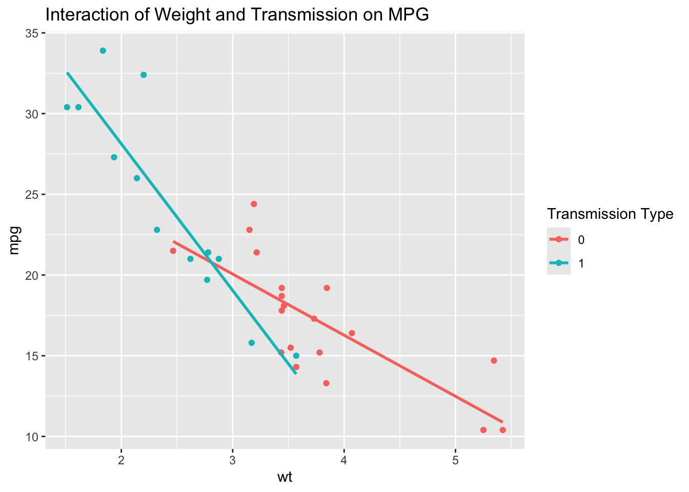

This plot helps to visually confirm the interaction effect by showing how the slope of mpg against wt differs depending on whether the car has an automatic or manual transmission.

9.6.1 Logistic Regression for Categorical Dependent Variables

Logistic regression is a statistical method used for modeling binary or categorical dependent variables. Unlike linear regression, which predicts a continuous outcome, logistic regression predicts the probability that a given observation falls into one of two categories. This method is particularly useful in scenarios where the outcome is categorical, such as predicting customer churn (yes/no), classifying emails as spam or not, or determining whether a patient has a disease (present/absent). The primary purpose of logistic regression is to model the relationship between a set of predictor variables and a binary outcome. It is widely used in various fields, including marketing, healthcare, and finance, to make predictions and classify outcomes based on input data. For example, a company might use logistic regression to predict whether a customer will renew their subscription based on factors such as previous purchase history, engagement level, and customer demographics.

The logistic regression model estimates the probability \(P(Y = 1)\) as a function of the predictors using the logit function:

\[ \text{logit}(P) = \log\left(\frac{P}{1-P}\right) = \beta_0 + \beta_1X_1 + \beta_2X_2 + \ldots + \beta_kX_k \]

In this equation, \(P\) represents the probability that the dependent variable equals 1, \(X_1, X_2, \ldots, X_k\) are the predictor variables, and \(\beta_0, \beta_1, \ldots, \beta_k\) are the coefficients to be estimated. The logit function transforms the probability into a log-odds scale, making it easier to model with a linear equation. In logistic regression, the coefficients represent the change in the log odds of the dependent variable for a one-unit change in the predictor variable. The odds can be interpreted as the ratio of the probability of the event occurring to the probability of it not occurring. The exponential of a coefficient \(\exp(\beta_j)\) gives the odds ratio, which indicates how the odds change with a one-unit increase in the predictor variable.

To implement logistic regression in R, consider the example of predicting whether a car has an automatic or manual transmission (am) based on various features in the mtcars dataset. The glm() function is used with the family = binomial argument to fit a logistic regression model:

logit_model <- glm(am ~ mpg + hp + wt, data = mtcars, family = binomial)
summary(logit_model)


Call:
glm(formula = am ~ mpg + hp + wt, family = binomial, data = mtcars)

Coefficients:
             Estimate Std. Error z value Pr(>|z|)  
(Intercept) -15.72137   40.00281  -0.393   0.6943  
mpg           1.22930    1.58109   0.778   0.4369  
hp            0.08389    0.08228   1.020   0.3079  
wt           -6.95492    3.35297  -2.074   0.0381 *
---
Signif. codes:  0 '***' 0.001 '**' 0.01 '*' 0.05 '.' 0.1 ' ' 1

(Dispersion parameter for binomial family taken to be 1)

    Null deviance: 43.2297  on 31  degrees of freedom
Residual deviance:  8.7661  on 28  degrees of freedom
AIC: 16.766

Number of Fisher Scoring iterations: 10

The coefficients in the model represent the log odds of the dependent variable being 1 (manual transmission) for each unit increase in the predictor variables. To interpret the effect size, these coefficients can be converted to odds ratios using:

exp(coef(logit_model))

 (Intercept)          mpg           hp           wt 
1.486947e-07 3.418843e+00 1.087513e+00 9.539266e-04

The p-values provided in the summary output help assess the significance of each predictor.

Evaluating the performance of the logistic regression model can be done using a confusion matrix, which compares the predicted classifications to the actual classifications. This helps in understanding how well the model is performing in terms of true positives, false positives, true negatives, and false negatives. In R, the table() function can be used to create a confusion matrix:

predicted <- ifelse(predict(logit_model, type = "response") > 0.5, 1, 0)
table(Predicted = predicted, Actual = mtcars$am)

         Actual
Predicted  0  1
        0 18  1
        1  1 12

Additionally, the ROC (Receiver Operating Characteristic) curve can be plotted to visualize the model’s performance across different threshold settings. The AUC (Area Under the Curve) provides a quantitative measure of model performance, with higher values indicating better performance. This can be implemented in R using the pROC package:

library(pROC)

Type 'citation("pROC")' for a citation.


Attaching package: 'pROC'

The following objects are masked from 'package:stats':

    cov, smooth, var

roc_curve <- roc(mtcars$am, predict(logit_model, type = "response"))

Setting levels: control = 0, case = 1

Setting direction: controls < cases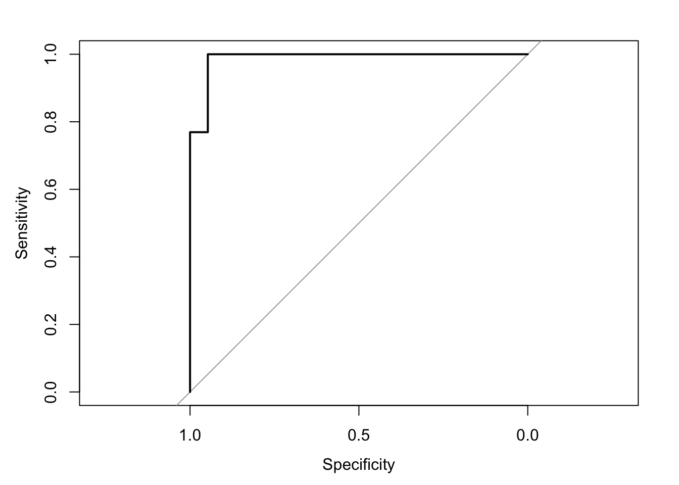

plot(roc_curve)

auc(roc_curve)

Area under the curve: 0.9879

Understanding and applying logistic regression allows for effective modeling and interpretation of scenarios where the outcome variable is categorical, offering valuable insights for decision-making and predictive analytics.

9.7 Advanced Techniques for Categorical Data

When working with categorical data, particularly variables with high cardinality, traditional methods like one-hot encoding can lead to an overwhelming increase in the number of variables, making models computationally expensive and prone to overfitting. High cardinality refers to categorical variables that have a large number of unique levels or categories. To address this, advanced techniques such as feature hashing can be employed.

Feature hashing, also known as the “hashing trick,” is a technique that converts high-cardinality categorical variables into a fixed number of features using a hash function. This reduces dimensionality and makes it possible to manage variables with many categories more efficiently. However, the technique introduces the possibility of hash collisions and reduces interpretability.

Caution

Handling high-cardinality categorical data is a complex subject. While feature hashing provides one solution, other techniques such as entity embeddings or weight-of-evidence encoding may be more suitable depending on the problem. Implementation of these methods is beyond the scope of this text. Students are encouraged to research their specific problem carefully and experiment with different approaches, or consult a professional if the project requires specialized expertise.

Tree-based models, such as decision trees and random forests, offer another approach for handling categorical data. Decision trees are a non-parametric, tree-structured method used for both classification and regression tasks, and they naturally handle categorical data without the need for encoding. Decision trees are easily interpretable and manage both categorical and continuous data, but they can be prone to overfitting and are sensitive to noisy data.

Random forests, an ensemble method that builds multiple decision trees and merges them to improve accuracy and reduce overfitting, are particularly effective at handling categorical data, even with high cardinality. While random forests handle large datasets with high dimensionality and provide feature importance metrics, they are less interpretable than single decision trees and require more computational resources.

Gradient Boosting Machines (GBMs) are another ensemble learning technique that builds models sequentially, with each new model correcting the errors of the previous ones. GBMs are effective at handling categorical data and improving model performance. GBMs offer high predictive accuracy and can handle complex models with interaction effects, but they require careful tuning of hyperparameters and are more computationally intensive, with a risk of overfitting if not properly regularized.

By employing these advanced techniques, such as feature hashing, decision trees, random forests, and gradient boosting machines, you can effectively manage high cardinality, improve model performance, and gain deeper insights from categorical data in a variety of applications.