Lecture 3: Fitting a Simple Linear Regression Model

Introduction to Simple Linear Regression

• Objective:
  • The goal of this lecture is to fit a simple linear regression model to predict Energy Efficiency (MPG) using Horsepower as the predictor variable. This allows us to quantify the relationship between the two variables and determine how changes in Horsepower affect MPG.
  • Simple linear regression models the linear relationship between a single predictor and a response variable.
• Why This Is Important:
  • By fitting a linear regression model, we can make predictions about MPG based on Horsepower. This analysis is crucial in automotive design, where fuel efficiency is often a trade-off with performance.
• Key Learning Outcomes:
  • By the end of this lecture, students will be able to:
    • Fit a simple linear regression model using R.
    • Interpret the regression output, including coefficients, p-values, and R-squared values.
    • Visualize the regression line on a scatter plot.

Fitting the Simple Linear Regression Model

Code Chunk: Fitting the Linear Regression Model

# Fit the simple linear regression model
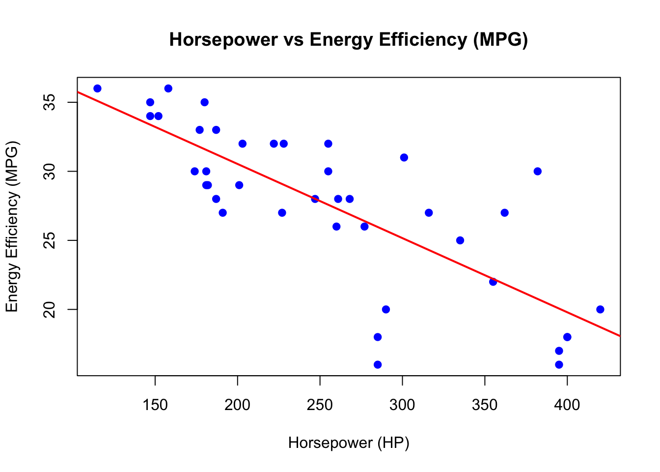
model <- lm(`Energy Efficiency (MPG)` ~ Horsepower, data = car_data_clean)

# Output the summary of the model
summary(model)

Call:
lm(formula = `Energy Efficiency (MPG)` ~ Horsepower, data = car_data_clean)

Residuals:
   Min     1Q Median     3Q    Max 
-9.968 -1.966  0.683  1.933  9.241 

Coefficients:
             Estimate Std. Error t value Pr(>|t|)    
(Intercept) 41.270812   1.864643  22.133  < 2e-16 ***
Horsepower  -0.053695   0.006956  -7.719 2.68e-09 ***
---
Signif. codes:  0 '***' 0.001 '**' 0.01 '*' 0.05 '.' 0.1 ' ' 1

Residual standard error: 3.689 on 38 degrees of freedom
Multiple R-squared:  0.6106,    Adjusted R-squared:  0.6003 
F-statistic: 59.58 on 1 and 38 DF,  p-value: 2.677e-09

Breaking Down the Code

• lm(): The lm() function in R fits a linear regression model. The formula Energy Efficiency (MPG) ~ Horsepower specifies that Energy Efficiency (MPG) is the response variable, and Horsepower is the predictor variable.
• summary(): This function provides detailed output about the fitted model, including the coefficients, standard errors, t-values, p-values, and the overall goodness-of-fit measures.

Interpreting the Model Output

• Coefficients:
  • Intercept (\(\beta_0\)): The intercept represents the expected MPG when Horsepower is 0. This value shows the baseline fuel efficiency when no horsepower is present.
  • Slope (\(\beta_1\)): The slope tells us how MPG changes for every one-unit increase in Horsepower. A negative slope indicates that higher horsepower leads to lower fuel efficiency.
• Significance of the Coefficients:
  • The p-value for the slope (Horsepower) will tell us whether the relationship between Horsepower and MPG is statistically significant. A small p-value (typically < 0.05) would indicate that horsepower significantly affects fuel efficiency.
• Goodness of Fit:
  • R-squared: Measures how much of the variation in MPG can be explained by Horsepower. Higher values indicate that the model explains a greater proportion of the variance.
  • Residual Standard Error: Represents the average distance between the observed and predicted values of MPG.

Visualizing the Fitted Regression Line

Code Chunk: Plotting the Regression Line

# Scatter plot with regression line
plot(car_data_clean$Horsepower, car_data_clean$`Energy Efficiency (MPG)`, 
     main = "Horsepower vs Energy Efficiency (MPG)",
     xlab = "Horsepower (HP)",
     ylab = "Energy Efficiency (MPG)",
     pch = 19, col = "blue")

# Add the regression line to the scatter plot
abline(model, col = "red", lwd = 2)

Breaking Down the Code

• plot(): Creates a scatter plot to visualize the relationship between Horsepower and MPG.
• abline(model): Adds the fitted regression line to the scatter plot. This line represents the best-fit linear relationship between Horsepower and MPG.

Visual Interpretation:

• The red regression line helps visualize the negative relationship between Horsepower and MPG. As Horsepower increases, MPG decreases, which aligns with the output of the linear regression model.

Summary and Next Steps

• Summary:
  • In this lecture, we built a simple linear regression model to quantify the relationship between Horsepower and MPG.
  • We interpreted the coefficients, p-values, and R-squared values to understand the strength and significance of the relationship.
  • We also visualized the regression line to see how well the model fits the data.
• Next Steps:
  • In the next lecture, we will evaluate the assumptions of the linear regression model by performing residual diagnostics. This will help us ensure that the model is appropriate for the data and does not violate key assumptions like linearity and homoscedasticity.

Assignment for Students:

1. Fit a simple linear regression model using Horsepower to predict MPG.
2. Generate the summary output and interpret the coefficients, p-values, and R-squared values.
3. Create a scatter plot with the fitted regression line.
4. Submit a brief explanation of your results, focusing on the significance of the relationship between Horsepower and MPG.