Chapter 7 Introduction to Linear Regression
PRELIMINARY AND INCOMPLETE
7.1 Case Study: Linear Regression Modeling of House Prices in Windsor
In this case study, we will utilize the Housing dataset from the Ecdat package to model house prices in the City of Windsor using linear regression. The objective of this study is to determine which variables most significantly impact house prices.
Description of the Data
The Housing dataset contains data about various properties in the City of Windsor, Canada. Each row corresponds to a house and the dataset includes variables such as lot size, the number of bedrooms, and the price of the house.
Let’s load and inspect the first few rows of the data.
##   price lotsize bedrooms bathrms stories driveway recroom fullbase gashw airco
## 1 42000    5850        3       1       2      yes      no      yes    no    no
## 2 38500    4000        2       1       1      yes      no       no    no    no
## 3 49500    3060        3       1       1      yes      no       no    no    no
## 4 60500    6650        3       1       2      yes     yes       no    no    no
## 5 61000    6360        2       1       1      yes      no       no    no    no
## 6 66000    4160        3       1       1      yes     yes      yes    no   yes
##   garagepl prefarea
## 1        1       no
## 2        0       no
## 3        0       no
## 4        0       no
## 5        0       no
## 6        0       no
Step 1: Explore the Data
We’ll begin by exploring the data to get an understanding of the variables and their relationships.
Summary Statistics
To get an overview of the data, we’ll use the describe function from the psych package.
##          vars   n     mean       sd      se
## price       1 546 68121.60 26702.67 1142.77
## lotsize     2 546  5150.27  2168.16   92.79
## bedrooms    3 546     2.97     0.74    0.03
## bathrms     4 546     1.29     0.50    0.02
## stories     5 546     1.81     0.87    0.04
## garagepl   11 546     0.69     0.86    0.04
Scatter plots of Numeric Variables vs. Housing Price
Now, we’ll visualize the relationship between each numeric variable and the housing price using scatter plots.
Housing %>%
  pivot_longer(cols = -c(price,!where(is.numeric)), names_to = "variable", values_to = "value") %>%
  ggplot(aes(x=value, y=price, color =fullbase)) +
    geom_point() +
    facet_wrap(~variable, scales="free") +
    geom_smooth(method = "lm",se = FALSE) +
    theme_minimal() +
    labs(title = "Scatter plots of Numeric Variables vs. Housing Price")
## `geom_smooth()` using formula = 'y ~ x'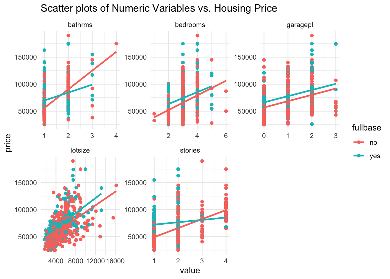
Step 2: Estimate Initial Model
We’ll use the lm function to estimate a model using all variables in the dataset to predict the house price.
| Observations | 546 |
| Dependent variable | price |
| Type | OLS linear regression |
| F(21,524) | 53.51 |
| R² | 0.68 |
| Adj. R² | 0.67 |
| Est. | S.E. | t val. | p | |
|---|---|---|---|---|
| (Intercept) | -2927.59 | 3989.94 | -0.73 | 0.46 |
| lotsize | 2.95 | 0.43 | 6.83 | 0.00 |
| bedrooms | 1029.66 | 1292.86 | 0.80 | 0.43 |
| bathrms | 17703.23 | 2079.88 | 8.51 | 0.00 |
| stories | 6845.82 | 1137.17 | 6.02 | 0.00 |
| drivewayyes | 7173.28 | 2439.35 | 2.94 | 0.00 |
| recroomyes | 1222.95 | 3299.35 | 0.37 | 0.71 |
| fullbaseyes | 3808.34 | 7903.27 | 0.48 | 0.63 |
| gashwyes | 7550.94 | 4019.13 | 1.88 | 0.06 |
| aircoyes | 12610.51 | 2042.54 | 6.17 | 0.00 |
| garagepl | 3687.41 | 1059.70 | 3.48 | 0.00 |
| prefareayes | 9020.09 | 2268.30 | 3.98 | 0.00 |
| lotsize:fullbaseyes | 1.22 | 0.77 | 1.59 | 0.11 |
| bedrooms:fullbaseyes | 1753.10 | 2244.27 | 0.78 | 0.44 |
| bathrms:fullbaseyes | -6636.71 | 3018.23 | -2.20 | 0.03 |
| stories:fullbaseyes | -1295.80 | 2258.51 | -0.57 | 0.57 |
| drivewayyes:fullbaseyes | -1360.09 | 4464.07 | -0.30 | 0.76 |
| recroomyes:fullbaseyes | 3928.59 | 4060.41 | 0.97 | 0.33 |
| fullbaseyes:gashwyes | 12686.80 | 6901.43 | 1.84 | 0.07 |
| fullbaseyes:aircoyes | -765.35 | 3212.87 | -0.24 | 0.81 |
| fullbaseyes:garagepl | 1568.08 | 1744.03 | 0.90 | 0.37 |
| fullbaseyes:prefareayes | 565.00 | 3437.07 | 0.16 | 0.87 |
| Standard errors: OLS |
Step 3: Variable Selection
Using the step function, we’ll remove all variables that are not significant at the 10% significance level.
| Observations | 546 |
| Dependent variable | price |
| Type | OLS linear regression |
| F(14,531) | 80.75 |
| R² | 0.68 |
| Adj. R² | 0.67 |
| Est. | S.E. | t val. | p | |
|---|---|---|---|---|
| (Intercept) | -3236.43 | 3600.46 | -0.90 | 0.37 |
| lotsize | 2.87 | 0.42 | 6.88 | 0.00 |
| bedrooms | 1625.18 | 1039.94 | 1.56 | 0.12 |
| bathrms | 17378.48 | 1993.21 | 8.72 | 0.00 |
| stories | 6365.54 | 944.92 | 6.74 | 0.00 |
| drivewayyes | 6798.72 | 2030.01 | 3.35 | 0.00 |
| recroomyes | 3890.67 | 1899.76 | 2.05 | 0.04 |
| fullbaseyes | 4807.70 | 4914.95 | 0.98 | 0.33 |
| gashwyes | 7304.63 | 3977.70 | 1.84 | 0.07 |
| aircoyes | 12463.47 | 1546.60 | 8.06 | 0.00 |
| garagepl | 4295.51 | 835.13 | 5.14 | 0.00 |
| prefareayes | 9400.45 | 1684.88 | 5.58 | 0.00 |
| lotsize:fullbaseyes | 1.48 | 0.66 | 2.24 | 0.03 |
| bathrms:fullbaseyes | -5788.40 | 2845.82 | -2.03 | 0.04 |
| fullbaseyes:gashwyes | 13260.46 | 6681.93 | 1.98 | 0.05 |
| Standard errors: OLS |
Step 4: Plot Actual vs. Fitted
Now, let’s visualize how well our model’s predictions match the actual prices.
predicted_prices <- predict(model_stepwise)

ggplot(Housing, aes(x = price, y = predicted_prices)) +
  geom_point(alpha = 0.5) +
  geom_smooth(se = FALSE, color = "black") +
  geom_abline(slope = 1, intercept = 0, color = "red") +
  theme_minimal() +
  labs(title = "Actual vs. Fitted Prices", x = "Actual Price", y = "Fitted Price")
## `geom_smooth()` using method = 'loess' and
## formula = 'y ~ x'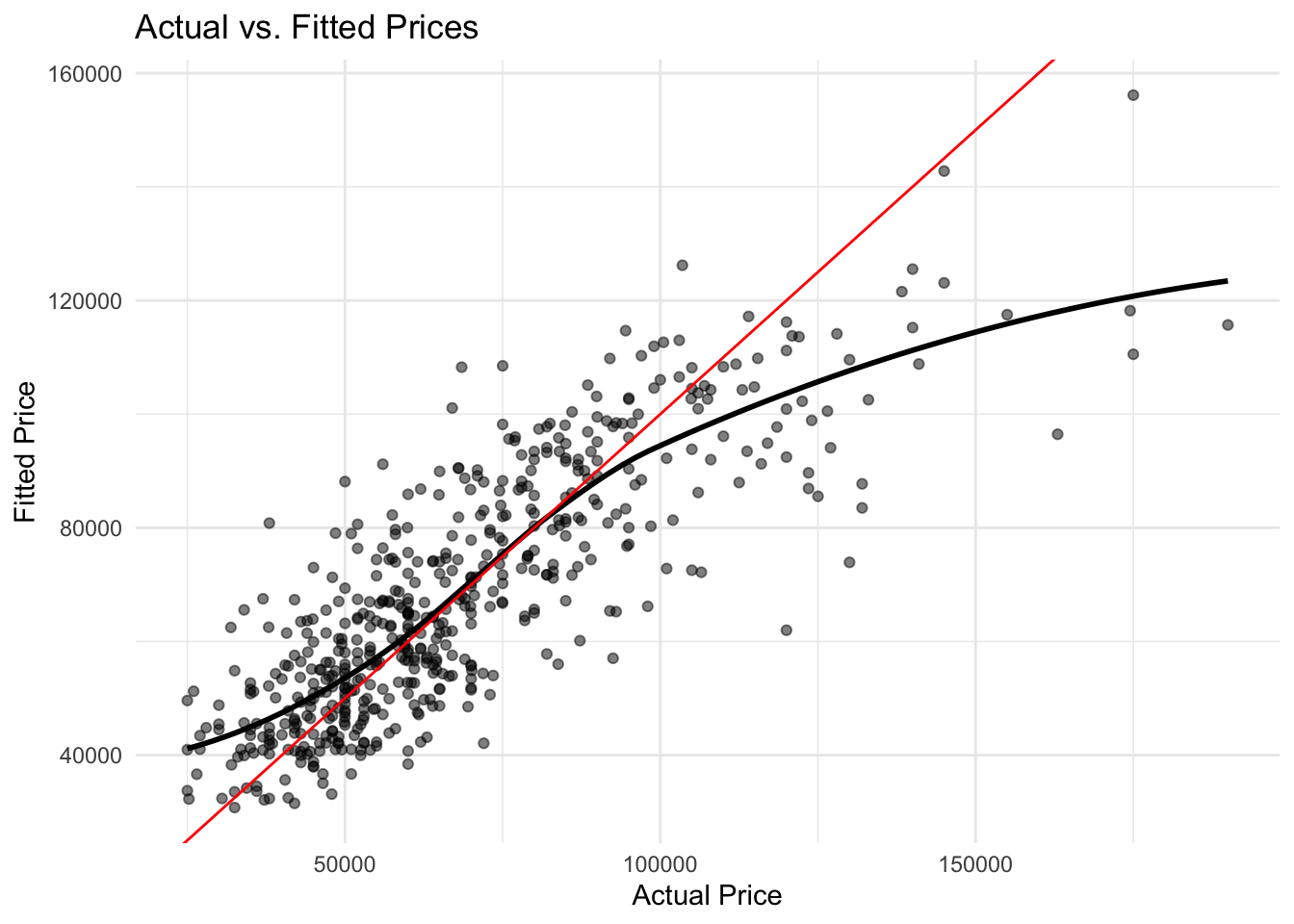
Step 5: Re-estimate with a Log-Log Model
A log-linear model can be useful when the underlying relationship appears to be nonlinear. In the next model, we will take the natural log of both price and lotsize.
model_initial_log <-
  lm(log(price) ~ (. - lotsize + log(lotsize)) * fullbase,
     data = Housing)
model_log <- step(model_initial_log, trace = 0)
summ(model_log)| Observations | 546 |
| Dependent variable | log(price) |
| Type | OLS linear regression |
| F(13,532) | 90.94 |
| R² | 0.69 |
| Adj. R² | 0.68 |
| Est. | S.E. | t val. | p | |
|---|---|---|---|---|
| (Intercept) | 7.80 | 0.22 | 35.78 | 0.00 |
| bedrooms | 0.03 | 0.01 | 2.29 | 0.02 |
| bathrms | 0.20 | 0.03 | 7.33 | 0.00 |
| stories | 0.09 | 0.01 | 6.71 | 0.00 |
| drivewayyes | 0.11 | 0.03 | 3.98 | 0.00 |
| recroomyes | 0.06 | 0.03 | 2.18 | 0.03 |
| fullbaseyes | 0.19 | 0.05 | 3.41 | 0.00 |
| gashwyes | 0.13 | 0.05 | 2.32 | 0.02 |
| aircoyes | 0.17 | 0.02 | 7.79 | 0.00 |
| garagepl | 0.05 | 0.01 | 4.27 | 0.00 |
| prefareayes | 0.14 | 0.02 | 6.04 | 0.00 |
| log(lotsize) | 0.29 | 0.03 | 10.86 | 0.00 |
| bathrms:fullbaseyes | -0.07 | 0.04 | -1.78 | 0.08 |
| fullbaseyes:gashwyes | 0.15 | 0.09 | 1.63 | 0.10 |
| Standard errors: OLS |
predicted_prices <- predict(model_log)

ggplot(Housing, aes(x = log(price), y = predicted_prices)) +
  geom_point(alpha = 0.5) +
  geom_smooth(se = FALSE, color = "black") +
  geom_abline(slope = 1, intercept = 0, color = "red") +
  theme_minimal() +
  labs(title = "Actual vs. Fitted Prices", x = "Actual Price", y = "Fitted Price")
## `geom_smooth()` using method = 'loess' and
## formula = 'y ~ x'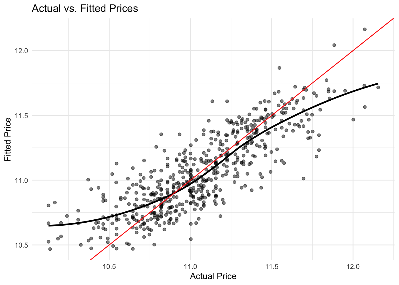
Step 6: Interpret the Model
Certainly, when modeling with the natural logarithm of the dependent variable, interpreting coefficients can be approached in terms of percentage changes. Here’s the interpretation of the coefficients in terms of percentage changes:
In the OLS regression model for house prices based on 546 observations:
- For every additional bedroom, the house price is expected to increase by approximately \(100 \times 0.03 = 3\%\), holding other variables constant.
- Each additional bathroom is associated with a \(100 \times 0.20 = 20\%\) increase in the house price, all else being equal.
- An additional story raises the house price by \(100 \times 0.09 = 9\%\).
- Having a driveway boosts the house price by about \(100 \times 0.11 = 11\%\).
- A recreation room elevates the price by \(100 \times 0.06 = 6\%\).
- Houses with a full basement see a \(100 \times 0.19 = 19\%\) price hike.
- The presence of gas hot water heating increases the price by \(100 \times 0.13 = 13\%\).
- Air conditioning contributes to a \(100 \times 0.17 = 17\%\) price rise.
- Each additional garage place augments the price by \(100 \times 0.05 = 5\%\).
- Being in a preferred area is associated with a \(100 \times 0.14 = 14\%\) price premium.
- A 1% increase in lot size leads to a \(0.29 \times 1\% = 0.29\%\) increase in the house price.
Interactions, like bathrms:fullbaseyes and fullbaseyes:gashwyes, complicate the percentage interpretation because they denote the change in the price percentage due to the combined effect of both features, rather than their individual influences. For instance, the bathrms:fullbaseyes coefficient suggests that having both an additional bathroom and a full basement reduces the combined expected price increase by 7%, compared to when these features are considered separately.
In essence, the model’s coefficients give insights into the relative importance and effect of different house features on its price, with features like the number of bathrooms, air conditioning, and location in a preferred area having substantial impacts.
7.2 Case Study Assignments
7.2.1 Wine Quality
This case study applies the linear regression to data from Portuguese wine producers. The dataset is available at https://ljkelly3141.github.io/ABE-Book/data/winequality-red_small.csv, Cortez, Paulo, Cerdeira, A., Almeida, F., Matos, T., and Reis, J.. (2009).5
Case Background
As a vineyard owner, you want to develop an objective methode of evaluating your wines. To understand what factors contribute most significantly to wine quality, we will use a dataset that contains physicochemical attributes of wines and their corresponding quality ratings. Leveraging this dataset, our aim is to determine which characteristics of a wine lead to high-quality ratings.
Description of the Data
The dataset contains red wine samples. The data has been sourced from the north of Portugal. There are several variables in the dataset, including:
| Variable | Description |
|---|---|
| residual sugar | Amount of sugar remaining after fermentation stops, rare to find wines with less than 1 gram/liter |
| pH | Describes how acidic or basic a wine is on a scale from 0 (very acidic) to 14 (very basic); most wines are between 3-4 |
| sulphates | Wine additive that can contribute to sulfur dioxide gas (S02) levels, acts as an antimicrobial and antioxidant |
| alcohol | Alcohol content of the wine |
| quality | Wine quality as assessed by experts, score between 0 and 10 |
These descriptions are based on the initial attributes provided in the dataset.
Instructions
Set Up
Before beginning the analysis, it’s essential to have all the necessary packages installed and loaded. If you haven’t already, make sure to install and load the pacman package using if(!require(pacman)) install.packages("pacman"). Once you’ve confirmed that pacman is available, load the required packages with pacman::p_load(tidyverse, jtools, psych).
Loading the Data
To kick off the actual analysis, you’ll be working with a dataset available in a comma-separated values (CSV) format. Use the read.csv() function and the provided URL to load this dataset into a variable named wine_data, i.e.
wine_data <- read.csv("https://ljkelly3141.github.io/ABE-Book/data/winequality-red_small.csv",
                      header=TRUE)
Data Cleaning
After you’ve successfully loaded the dataset, some minor cleaning will be necessary. Specifically, you should remove an index variable named X from the dataset. The select() function from the dplyr package can help you achieve this.
Summary Statistics
Once your data is cleaned and ready, it’s important to gain a basic understanding of its structure and characteristics. Utilize the describe() function to get an overview and summary statistics of all variables in your dataset.
Data Visualization
Next, to visualize the relationships between variables in your dataset, employ the pairs.panels() function. This will generate pairwise plots and give you insights into the interactions and correlations among the dataset’s variables.
Regression Analysis
Now, you’ll dive deeper into the core analysis. To understand the relationship between wine quality and other factors in the dataset, perform a linear regression. Use the lm() function to regress the quality variable against all other variables present in your dataset.
Residual Analysis
Once your regression model is set, it’s essential to assess its accuracy and potential errors. First, you will create a new data frame named wine.lm.values. This frame will store three main columns: actual quality values, fitted values from your regression model, and the residuals (errors) from your predictions, i.e.
wine.lm.values <- data.frame(check.names = FALSE,
           "Actual Values" = wine_data$quality,
           "Fitted Values" = wine.lm$fitted.values,
           "Residauls" = wine.lm$residuals)
To visualize the residuals and understand the model’s behavior better, plot the residuals against the fitted values using ggplot2. The aim is to see if the residuals scatter randomly around zero, which would indicate a well-fitted model. Here is an example of how to plot the residuals vs fitted values
wine.lm.values %>% ggplot(aes(y=`Residauls`,x=`Fitted Values`)) +
  geom_point() +
  geom_abline(intercept = 0,slope = 0) +
  geom_smooth(se=FALSE) +
  theme_minimal() +
  ggtitle("Residual vs. Fitted Values")
Actual vs. Predicted
Furthermore, you’ll compare the actual wine quality values to the values predicted by your model. Create a scatter plot where the x-axis represents the actual quality values and the y-axis represents the fitted values. If your model is accurate, most points should cluster around a 45-degree line.
wine.lm.values %>% ggplot(aes(x=`Actual Values`,y=`Fitted Values`)) +
  geom_point() +
  geom_abline(intercept = 0,slope = 1,colour="red") +
  theme_minimal() +
  ggtitle("Actual vs. Fitted Values")
Interpretations & Conclusions
After all the analysis, it’s time for reflection and interpretation. Please answer these questions, and provide your recommendations.
Questions:
- Reflect on the summary statistics: What did you observe about the dataset?
- What insights did the pairwise relationships provide regarding correlations between variables?
- Analyze the regression results: Which variables significantly predict wine quality? What did the R-squared value reveal?
- Assess the residuals vs. fitted values plot: Were the residuals random or was there a discernable pattern?
- For the actual vs. predicted plot, did the points tend to cluster around the 45-degree line? What might that suggest?
Recommendations & Confidence:
Finally, based on your analysis, provide your recommendations: - Propose recommendations on how to potentially improve wine quality. - Highlight any variables that may warrant more attention during the wine production process. - Reflect on the confidence level you hold regarding the model’s validity and predictions. Were there aspects of the model that made you more or less confident in its results?
Cortez, Paulo, Cerdeira, A., Almeida, F., Matos, T., and Reis, J.. (2009). Wine Quality. UCI Machine Learning Repository. https://doi.org/10.24432/C56S3T.↩︎