Chapter 6 Analysis of Variance (ANOVA)
6.1 Case Study Examples
6.1.1 Test in E-Commerce Data (ANOVA)
Introduction
This case study examines the application of the Analysis of Variance (ANOVA) test using R on a real-world dataset. The dataset used in this case study is the Online Retail II data set available from the UCI Machine Learning Repository. It is a transactional data set which contains all the transactions occurring for a UK-based and registered, non-store online retail between 01/12/2009 and 09/12/2011.
The main question we want to answer in this case study is: “Is there a significant difference in the average transaction amount across different countries?” To answer this question, we will conduct an Analysis of Variance (ANOVA) test, a statistical method used to test differences between two or more means. It can be viewed as an extension of the t-test.
Objective
Conduct an analysis of variance (ANOVA) to answer the question: “Is there a significant difference in the quantity of products purchased across different countries?” without utilizing the builtin anova() command.
Loading Necessary Packages
This case will use the dplyr package. The dplyr package is a popular data manipulation package in R. It provides a set of tools that are specifically designed to work with data frames, making it incredibly easy to transform and summarize your data. It’s part of the larger tidyverse collection of packages, which are designed to work together in data analysis.
Description of the Data
# Load the data
data <- read.xlsx("https://ljkelly3141.github.io/ABE-Book/data/online_retail_II.xlsx")

# Print first few rows of the dataset
head(data)
## Invoice StockCode Description Quantity InvoiceDate
## 1 489434 85048 15CM CHRISTMAS GLASS BALL 20 LIGHTS 12 40148.32
## 2 489434 79323P PINK CHERRY LIGHTS 12 40148.32
## 3 489434 79323W WHITE CHERRY LIGHTS 12 40148.32
## 4 489434 22041 RECORD FRAME 7" SINGLE SIZE 48 40148.32
## 5 489434 21232 STRAWBERRY CERAMIC TRINKET BOX 24 40148.32
## 6 489434 22064 PINK DOUGHNUT TRINKET POT 24 40148.32
## Price Customer.ID Country
## 1 6.95 13085 United Kingdom
## 2 6.75 13085 United Kingdom
## 3 6.75 13085 United Kingdom
## 4 2.10 13085 United Kingdom
## 5 1.25 13085 United Kingdom
## 6 1.65 13085 United KingdomHere is the description of relevant variables in the data set:
| Variable | Description |
|---|---|
| InvoiceNo | Invoice number. Nominal. A 6-digit integral number uniquely assigned to each transaction. |
| StockCode | Product (item) code. Nominal. A 5-digit integral number uniquely assigned to each distinct product. |
| Description | Product (item) name. Nominal. |
| Quantity | The quantities of each product (item) per transaction. Numeric. |
| InvoiceDate | Invoice date and time. Numeric. The day and time when a transaction was generated. |
| UnitPrice | Unit price. Numeric. Product price per unit in sterling (£). |
| CustomerID | Customer number. Nominal. A 5-digit integral number uniquely assigned to each customer. |
| Country | Country name. Nominal. The name of the country where a customer resides. |
Data Cleaning
Before performing an ANOVA test, it’s essential to clean the data. Let’s break down each step to clean and then summarize the data :
Step 1: Remove missing values
The first part of the code chunk removes rows that have missing values in the ‘CustomerID’ or ‘Description’ columns. This is achieved using the filter() function from the dplyr package.
The %>% operator is a pipe operator that takes the output of the code on its left and uses it as input for the function on its right. The filter() function is used to subset rows in a data frame based on a condition. The is.na() function checks for missing values, and the ! operator negates the condition. So filter(!is.na(CustomerID)) means “filter the data to include only the rows where ‘CustomerID’ is not missing”.
Step 2: Filter for positive quantities and prices
The second part of the code chunk filters the data to include only rows where ‘Quantity’ is greater than 0 and ‘UnitPrice’ is greater than 0.
This is again done using the filter() function. So filter(Quantity > 0) means “filter the data to include only the rows where ‘Quantity’ is greater than 0”.
Step 3: Calculate Total Amount of each Invoice
Here we will calculate the tot amount of each invoice. We will do so as follows:
data_final <- data_clean %>%
  mutate(TransTotal = Price * Quantity,
         InvoiceDate = convertToDate(InvoiceDate)) %>%
  group_by(Invoice) %>%
  mutate(InvoiceTotal = sum(TransTotal)) %>%
  distinct(Invoice, .keep_all = TRUE) %>%
  select(Invoice,InvoiceDate,InvoiceTotal,Country)
This is a bit much, so let’s break down the operations:
Initial Data Preparation: The
mutate()function is first employed on thedata_cleandataset to:- Calculate a new variable,
TransTotal, which is the product ofPriceandQuantity. - Convert the
InvoiceDateto a date format using a presumed functionconvertToDate().
- Calculate a new variable,
Grouping: The dataset is then grouped by the
Invoicecolumn usinggroup_by(Invoice). This means that any subsequent operations will be applied to each unique invoice separately.Summarizing Invoices: Within each unique invoice group, another
mutate()function calculates theInvoiceTotalwhich is the sum of all the transaction totals (TransTotal) within that particular invoice.Filtering Unique Invoices: The
distinct(Invoice, .keep_all = TRUE)function is applied to retain only unique invoices. The.keep_all = TRUEparameter ensures that all other columns (associated with that unique invoice) are retained.Selecting Relevant Columns: Finally, the
select()function is used to retain only the columnsInvoice,InvoiceDate,InvoiceTotal, andCountryin the final dataset.Previewing the Data: The last line,
head(data_final), is used to display the first six rows of thedata_finaldataset, providing a snapshot of the processed data.
Performing the ANOVA Test Manually
In R, we can calculate the ANOVA manually. Here are the steps:
Step 1: Calculate the overall and country level means
Calculate country invoice count ant average.
country.summary <- data_final %>%
  group_by(Country) %>%
  summarise(CountryCount = n(),
            CountryMean = mean(InvoiceTotal)) %>%
  arrange(desc(CountryCount))
country.summary
## # A tibble: 37 × 3
## Country CountryCount CountryMean
## <chr> <int> <dbl>
## 1 United Kingdom 17612 421.
## 2 Germany 347 583.
## 3 EIRE 316 1127.
## 4 France 236 620.
## 5 Netherlands 135 1991.
## 6 Sweden 68 782.
## 7 Spain 66 721.
## 8 Belgium 52 472.
## 9 Australia 40 786.
## 10 Portugal 40 596.
## # ℹ 27 more rowsFilter countries with too few invoices.
data_final <- data_final %>%
  group_by(Country) %>%
  mutate(CountryCount = n()) %>%
  filter(CountryCount>=50) %>%
  ungroup()

country.summary <- country.summary %>%
  filter(CountryCount>=50)
Calculate the overall mean.
## [1] 452.0799Step 2: Total Sum of Squares
Calculate the total sum of squared difference from the mean, i.e. \(\sum_{i=1}^{N}{(Y_i-\bar{Y})^2}\).
## [1] 15641663963Step 3: Within-group sum of squares
Calculate the Within-group sum of squares, i.e. \(SS_{w} = \sum_{k=1}^{G}{\sum_{i=1}^{N_k}{(Y_{ik}-\bar{Y_k})^2}}\). To do this in R, we will do this in two steps. First, we make a new variable that has the group mean of each observation.
data_final <- data_final %>%
  group_by(Country) %>%
  mutate(CountryMean = mean(InvoiceTotal)) %>%
  ungroup()
Then, we can simply sum the squared difference.
## [1] 15136264656Step 4: Between-group sum of squares
Calculate the Within-group sum of squares, i.e. \(SS_{b} = \sum_{k=1}^{G}{\sum_{i=1}^{N_k}{(\bar{Y_k}-\bar{Y})^2}}\).
## [1] 505399306Step 5: Degrees of freedom
Each of the sum of squares estimates have degrees of freedom.
## [1] 18824## [1] 7Step 6: Mean squares value
## [1] 804094## [1] 72199901Step 7: F-Stat
## [1] 89.79038Step 8: p-value
## [1] 2.720518e-129Conclusion
One-way ANOVA showed a significant difference between invoice totals across countries (F(7,18824)=89.79,p<.001).
Save the data for the next case
6.1.2 Test in E-Commerce Data (Checking our assumptions)
In this case, we will continue to work with the Online Retail II data set available from the UCI Machine Learning Repository.
Load and Clean Data
Load and clean the data as we did in the previous case.
Objective
Conduct an analysis of variance (ANOVA) to answer the question: “Is there a significant difference in the quantity of products purchased across different countries?” utilizing the built in anova() command and then check the vilidity of our conclution.
Instructions
Step 1: Conduct basic ANOVA
NOTE: You should always begin with exploratory analysis, but since this case is a continuation of the previous case, we can rely on the exploratory analysis conducted there.
##                Df    Sum Sq  Mean Sq F value Pr(>F)
## Country         7 5.054e+08 72199901   89.79 <2e-16 ***
## Residuals   18824 1.514e+10   804094
## ---
## Signif. codes:  0 '***' 0.001 '**' 0.01 '*' 0.05 '.' 0.1 ' ' 1
Step 2: Checking the Homogeneity of Variance Assumption
Draw a boxplot of invoice total by Country.
data_final %>% ggplot(aes(x=Country,y=InvoiceTotal)) +
  geom_boxplot() +
  scale_y_continuous(limits = c(0,2000))
## Warning: Removed 409 rows containing non-finite
## values (`stat_boxplot()`).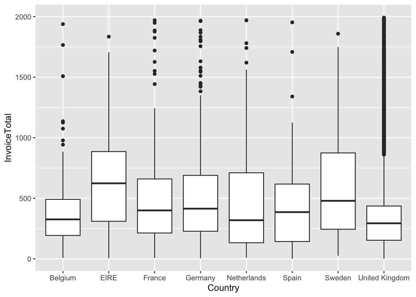
Use the Levene test of Homogeneity of Variance
## Warning in leveneTest.default(y = y, group = group, ...): group coerced to
## factor.
## Levene's Test for Homogeneity of Variance (center = median)
## Df F value Pr(>F)
## group 7 79.659 < 2.2e-16 ***
## 18824
## ---
## Signif. codes: 0 '***' 0.001 '**' 0.01 '*' 0.05 '.' 0.1 ' ' 1Both the boxplot and the Levene test indicate that the Homogeneity of Variance assumption is violated; thus, we should run the Welch one-way test.
##
##  One-way analysis of means (not assuming equal variances)
##
## data:  InvoiceTotal and Country
## F = 14.174, num df = 7.00, denom df = 313.66, p-value = 5.408e-16
The conclusion remains the same when we account for heteroscedasticity.
Step 3: Checking the Normality of Residuals
To evaluate the assumptions of our ANOVA model, one critical step is to determine whether the residuals are normally distributed. This assumption is essential as significant deviations can compromise the reliability of the model’s results.
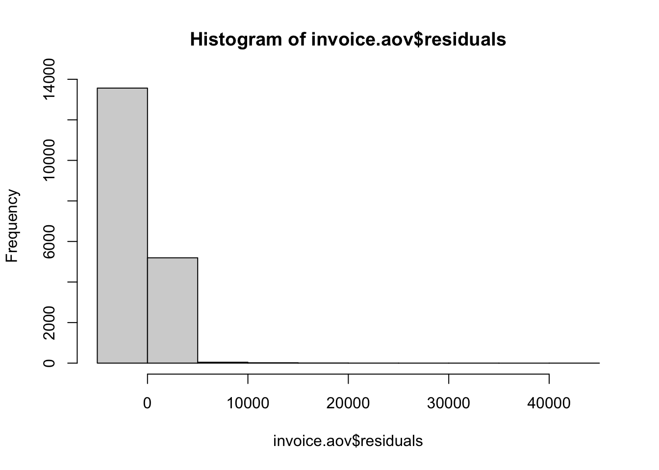 The histogram provides a visual representation of the distribution of residuals. A bell-shaped curve suggests a normal distribution, while noticeable deviations from this shape indicate non-normality.
# Q-Q plot of the residuals
qqnorm(invoice.aov$residuals)
qqline(invoice.aov$residuals) # Adding a reference line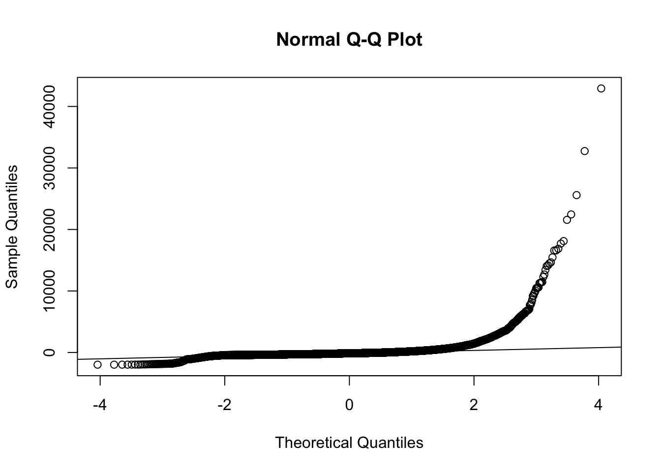 The Q-Q plot (quantile-quantile plot) is another graphical method to assess normality. If the residuals are normally distributed, the points should fall roughly along the diagonal reference line.
##
##  Shapiro-Wilk normality test
##
## data:  sample(invoice.aov$residuals, 5000)
## W = 0.26078, p-value < 2.2e-16
The Shapiro-Wilk test is a formal statistical test for normality. A significant p-value (typically less than 0.10, 0.05 or 0.01) suggests that the residuals do not follow a normal distribution.
All three of the above examinations indicate non-normality. As such we should use the Kruskal-Wallis test:
##
##  Kruskal-Wallis rank sum test
##
## data:  InvoiceTotal by Country
## Kruskal-Wallis chi-squared = 349.68, df = 7, p-value < 2.2e-16
The conclution remains the same.
6.2 Case Study Assignments
6.2.1 Analyzing Job Satisfaction Using ANOVA
Background:
As budding business analysts, understanding the nuances within Human Resource (HR) metrics is critical. HR analytics aids in deriving insights from data, which in turn informs decisions about process improvement. One dataset that can shed light on this is the “HR Analytics: Case Study” compiled by Bhanupratap Biswas in 2023.
In this assignment, you will dive deep into this dataset to discover if job satisfaction varies based on certain categorical variables: BusinessTravel, Department, and JobRole. here,compiled by Bhanupratap Biswas (2023).4
Objective:
Use ANOVA to determine if job satisfaction differs based on the categories BusinessTravel, Department, and JobRole.
Instructions:
Set Up:
Before beginning the analysis, it’s essential to have all the necessary packages installed and loaded. If you haven’t already, make sure to install and load the pacman package using if(!require(pacman)) install.packages("pacman"). Once you’ve confirmed that pacman is available, load the required packages with pacman::p_load(tidyverse, car, psych).
# Check to see if pacman is installed, and if not, install it.
if(!require(pacman)) install.packages("pacman")
# Load packages
pacman::p_load(tidyverse, car, psych)
Load the Data:
- Import the dataset using the following link:
Data Cleaning:
- Select the variables
BusinessTravel,Department,JobRole, andJobSatisfactionfor your analysis. - Identify and remove any observations with missing values.
To achieve this, use the following sample code:
# Selecting the required variables and storing in a new data frame
hr_clean <- hr_data %>%
  select(BusinessTravel, Department, JobRole, JobSatisfaction) %>%
  drop_na()
After executing these steps, review the hr_clean data frame to ensure it’s prepared for the subsequent analysis.
Summary Statistics:
- Compute the summary statistics of
JobSatisfactiongrouped by each of the categorical variables:BusinessTravel,Department, andJobRole. - Use the
psych::describe()function to obtain comprehensive statistics. - Present the results in a clear and organized manner.
Here is an example demonstrating one method of achieving this:
summary_by_travel <- hr_clean %>%
  group_by(BusinessTravel) %>%
  do(describe(.$JobSatisfaction,ranges = FALSE,skew = FALSE))

summary_by_travel
## # A tibble: 3 × 6
## # Groups: BusinessTravel [3]
## BusinessTravel vars n mean sd se
## <chr> <dbl> <dbl> <dbl> <dbl> <dbl>
## 1 Non-Travel 1 150 2.79 1.03 0.0842
## 2 Travel_Frequently 1 277 2.79 1.10 0.0661
## 3 Travel_Rarely 1 1043 2.70 1.11 0.0345The code above performs a series of operations on the hr_clean data frame with the aim of generating descriptive statistics for the JobSatisfaction variable, specifically grouped by the levels within BusinessTravel. Here’s a breakdown:
- The code starts with the
hr_cleandata frame. - It then groups the data by the
BusinessTravelvariable usinggroup_by(BusinessTravel). This ensures that any subsequent operations are performed separately for each unique value (or level) ofBusinessTravel. - The
do()function is then applied to each group. Inside thedo()function, thedescribe()function from thepsychpackage is used to compute a variety of descriptive statistics for theJobSatisfactionvariable within each group. - Additionally, certain statistics are omitted from the output by setting their respective arguments to
FALSE. In this case, the ranges (ranges = FALSE) and skewness (skew = FALSE) are excluded from the results. - The final output, which is a summarized table of the desired statistics for
JobSatisfactioncategorized byBusinessTravel, is stored in thesummary_by_travelobject.
Data Visualization:
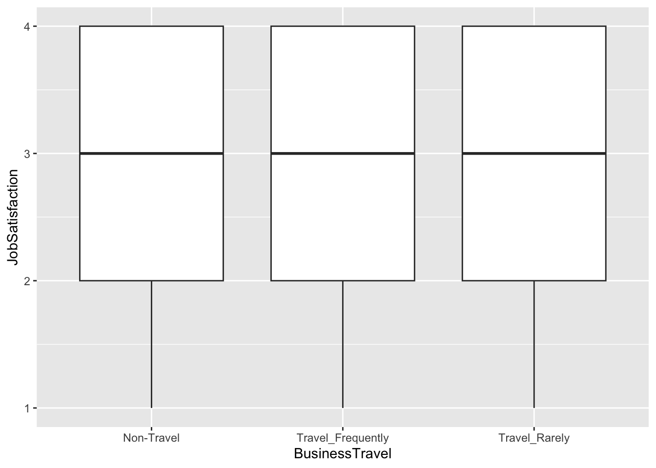
Create visualizations that display job satisfaction across the different categories of BusinessTravel, Department, and JobRole. Consider using boxplots for this purpose i.e.:
ANOVA Analysis:
Conduct ANOVA tests to determine if job satisfaction differs among the aforementioned categories.
Check Assumptions:
Before drawing any conclusions from your ANOVA results, validate the assumptions associated with the test. Specifically, check for:
- Homogeneity of variance across groups
- Normality of residuals for each ANOVA test
If assumptions are violated, determine the appropriate correction. What is the most approperiate model.
Questions to Answer:
- Based on your ANOVA results, does job satisfaction differ significantly across the categories of BusinessTravel, Department, and JobRole?
- Were the assumptions of ANOVA met for each test? If not, what implications might this have for your results?
- Which factor(s) – if any – would you recommend a business focus on if they want to improve job satisfaction?
Bhanupratap Biswas. (2023). HR Analytics: Case Study [Data set]. Kaggle. https://doi.org/10.34740/KAGGLE/DSV/5905686↩︎