Chapter 3 A First Look at R
This chapter will guide you through some basic syntax of R and illustrate how to conduct a simple data analysis of a dataset built directly into R called mtcars, which contains information on different cars from the 1970’s.
3.1 Understanding Data Frames
Before we delve into the mechanics of data analysis in R, let’s first understand what a data frame is. A data frame is a two-dimensional data structure. This is somewhat akin to a table in a spreadsheet or a SQL database, where information is organized in a grid of rows and columns:
Each row is an observation: Every row represents one single entity or observation. In the context of our
mtcarsdataset, each row corresponds to a unique car model, and every characteristic of that model (such as miles per gallon, horsepower, etc.) is listed in the same row.Each column is a variable: Every column represents a distinct variable or attribute of an observation. For example, in the
mtcarsdataset, thempgcolumn represents the miles per gallon variable, and thehpcolumn represents the horsepower variable. For every car model in the dataset (every row), there is a corresponding value in each column that characterizes that attribute for that specific car.Columns can be of different types, but data within each column is of the same type: In a data frame, each column can store a different type of data - numeric, factor, character, logical, etc. However, all data within a given column must be of the same type. For instance, all data within the
mpgcolumn is numeric, while data within a different column could be character type.
The structure of data frames makes it easy to organize and manipulate data in R, especially when dealing with datasets where each observation has multiple associated variables. Understanding how to work with data frames is a critical first step in becoming proficient in data analysis with R.
The mtcars dataset is a preloaded data frame in R, which is comprised of 32 rows, each representing a car model, and 11 columns detailing various attributes of these cars. To load the mtcars dataset into your working environment, use the data() function as follows:
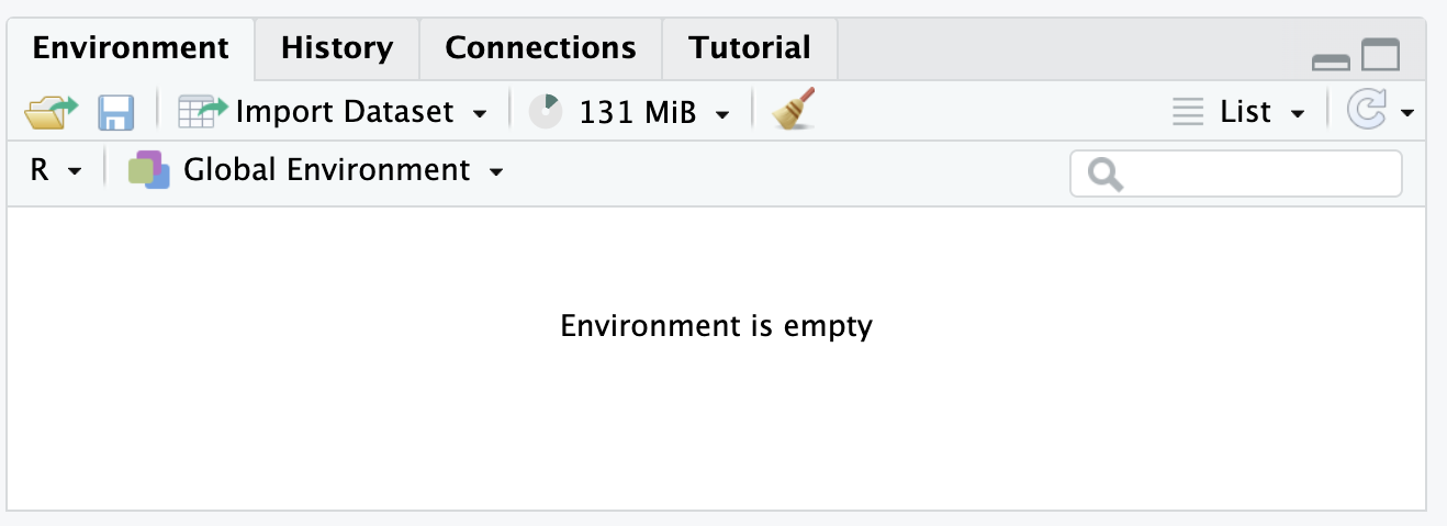
By invoking this command, you ensure that mtcars is available and ready to be utilized for your data analysis tasks. This method is preferred to directly referencing the dataset name, as it makes explicit the intention of loading the dataset. You will notice that mtcars is now listed in the Environment Panel.
3.2 Understanding the $ Operator in R
In R, we use the $ operator to access specific columns from a data frame. It’s a way of selecting a particular variable from a dataset. For example, if we want to work with the mpg (miles per gallon) variable from the mtcars dataset, we would do so as follows:
mtcars$mpg
3.3 Summarizing the miles per gallon variable
The summary() function in R provides a quick overview of the statistical properties of a dataset or a specific variable in the dataset. It displays the minimum value, first quartile (25th percentile), median (50th percentile), mean, third quartile (75th percentile), and maximum value of the variable in question.
In the code chunk above, we’re applying the summary() function to the mpg (miles per gallon) variable of the mtcars data frame. The $ operator is used to select the mpg variable from the mtcars data frame. The result of the summary() function is then assigned to the mpg_summary variable. The <- operator assigns the result of summary(mtcars$mpg) to this new variable.
In simpler terms, summary(mtcars$mpg) calculates the summary statistics of the mpg column in the mtcars data frame. The <- operator then stores this output in the mpg_summary variable. This assignment allows us to easily access the summary statistics later on by simply calling the mpg_summary variable, without having to rerun the summary(mtcars$mpg) function each time.
In R, both <- and = can be used as assignment operators. However, <- is more commonly used and is considered good practice because it is more readable, particularly when used within functions or in complex operations.
Note that <- directs the output of summary(mtcars$mpg) to mpg_summary; thus R does not display the results. We can display this summary by simply typing mpg_summary in the console and pressing enter (or return on a Mac):
##    Min. 1st Qu.  Median    Mean 3rd Qu.    Max.
##   10.40   15.43   19.20   20.09   22.80   33.90
After executing this command, you’ll see a summary of the mpg variable in your console. This summary will give you a quick sense of the central tendency, spread, and range of the mpg values in the mtcars data frame.
3.3.1 Plotting miles per gallon vs horsepower
Next, let’s analyize the relationship between miles per gallon (mpg) and horsepower (hp), To visualize this relationship, we use the plot() function. We pass information a function via argument, and in R, named arguments are an effective way to pass values to a function. For instance, when you execute the command plot(x = mtcars$hp, y = mtcars$mpg), x and y are named arguments. Their respective values are being assigned using the = operator, which clearly indicates that we are plotting horsepower (hp) on the x-axis and miles per gallon (mpg) on the y-axis. This explicit naming of arguments aids in understanding exactly what data is being plotted without necessarily knowing the default order of arguments in the plot() function. Note: you should not use <- in a function call.
plot(x = mtcars$hp,
     y = mtcars$mpg,
     xlab = "Horsepower",
     ylab = "Miles per Gallon",
     main = "Miles per Gallon vs Horsepower")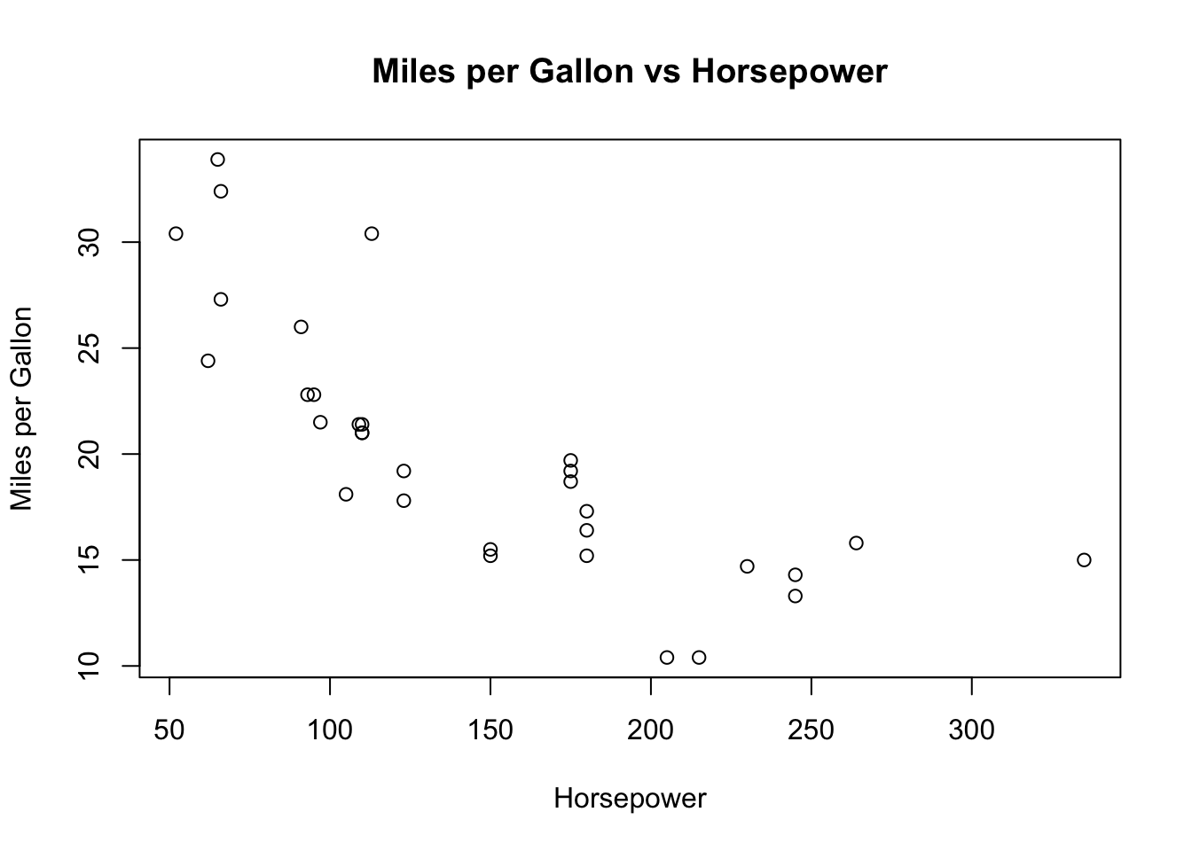
In R’s plot() function, you can add additional information to your plot by specifying parameters such as xlab, ylab, and main. Here’s what each of them does:
xlab: This parameter sets the label for the x-axis of the plot. The label is a text string that describes the data values represented along the x-axis. For example,xlab = "Horsepower"would label the x-axis as “Horsepower”.ylab: This parameter sets the label for the y-axis of the plot. Likexlab, the label provided here should describe the data values along the y-axis. For instance,ylab = "Miles per Gallon"would label the y-axis as “Miles per Gallon”.main: This parameter sets the main title of the plot. This title often summarizes what the plot represents. For example,main = "Miles per Gallon vs Horsepower"would set “Miles per Gallon vs Horsepower” as the title of the plot.
Thus, when we use plot(mtcars$hp, mtcars$mpg, xlab = "Horsepower", ylab = "Miles per Gallon", main = "Miles per Gallon vs Horsepower"), we are creating a scatterplot of hp against mpg, with appropriately labelled axes and a descriptive title. This helps make the plot more informative and easy to understand for anyone viewing it.
3.4 Fitting a Trend Line
Now, we’ll fit a trend line to our scatterplot to better visualize the relationship between hp and mpg. We’ll do this using the lm() function, which stands for “linear model”. The lm() function is a fundamental tool in R for linear regression analysis. It estimates the coefficients of a linear equation, involving one or more independent variables, that best predict the value of the dependent variable.
In the command above, we create a new variable fit that holds our linear model. We’re using the ~ symbol to denote the relationship between our response variable (mpg) and the predictor variable (hp). We also specify the dataset we’re working with using data = mtcars.
After fitting the model, we plot the points and add the fitted line using the abline() function:
plot(x = mtcars$hp,
     y = mtcars$mpg,
     xlab ="Horsepower",
     ylab = "Miles per Gallon",
     main = "Miles per Gallon vs Horsepower")
abline(fit, col="red")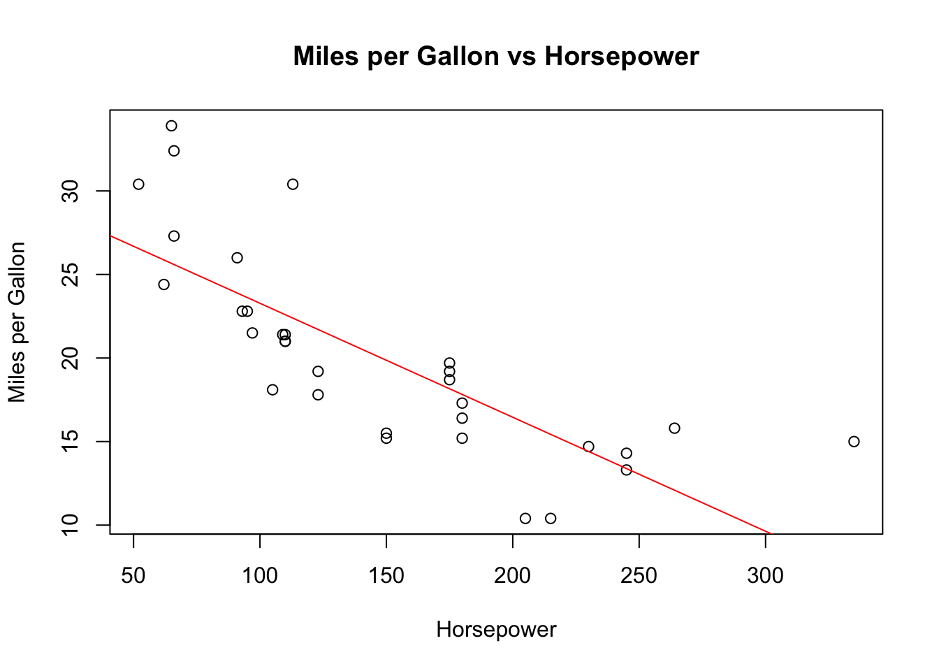
The abline() function draws a straight line on the current plot. By passing fit as an argument to abline(), we add the fitted line from our linear model to the scatter plot.
And there you have it! By learning these fundamental operations, you’ve conducted a basic analysis of the mtcars dataset using base R. This serves as a stepping stone to more complex tasks and analyses in R. Continue practicing, building upon these basics, and you’ll soon find yourself confidently navigating the extensive capabilities of R.