Chapter 4 Getting Started with R
PRELIMINARY AND INCOMPLETE
In this chapter, we will cover the basics of R programming, including functions, packages, comments, variables, data frames, lists, and formulas. We will also introduce important programming concepts like writing scripts, using loops and conditional statements, and creating functions.
4.1 Commands and Calculations
In this section, we will explore interacting with the R programming environment, performing simple calculations, and storing numeric values as variables.
4.1.1 Typing Commands at the R Console
R is an interactive language that lets you type commands directly into its console. When you type a command at the R prompt and press “Enter”, R immediately provides the output. For instance, if you use the print() function as shown below, R will return Hello, World! in the console.
## [1] "Hello, World!"4.1.2 Doing Simple Calculations with R
R serves as both a programming language and a powerful calculator. You can perform basic arithmetic operations such as addition, subtraction, multiplication, division, and exponentiation. For instance, when you type 3 * 5 in the R console, as shown below, you will get 15 - the product of 3 and 5.
## [1] 154.1.3 Storing a Number As a Variable
R enables you to store a numeric value as a variable for later use. This is accomplished using the assignment operator <-. For example, x <- 10 assigns the value 10 to the variable x. Once a value is stored as a variable, you can use it in future calculations. For instance, if you type x * 2 after assigning 10 to x, as shown below, R will return 20. This functionality is especially useful for performing complex operations and managing large datasets.
## [1] 204.2 Functions
Functions are an essential part of any programming language, including R. They allow you to encapsulate a set of instructions into a reusable block of code. This not only promotes code organization but also makes your programs more modular and easier to maintain. In this section, we will explore the concept of functions in R and how they can be used to perform calculations and streamline your workflow.
4.2.1 Using Functions to Do Calculations
One of the primary use cases of functions in R is to perform calculations. Instead of writing the same set of instructions repeatedly, you can use built-in functions to perform common calculations. In this example, we will use the mean() and sd() functions to calculate the mean and standard deviation of a variable in the mtcars dataset.
# Load the mtcars dataset
data(mtcars)

# Calculate the mean of the mpg variable
mpg_mean <- mean(mtcars$mpg)
print(mpg_mean)
## [1] 20.09062## [1] 6.026948In the above code chunk, we first load the mtcars dataset using the data() function. Then, we use the mean() function to calculate the mean of the mpg variable in the mtcars dataset. The mean() function takes a numeric vector as input and returns the arithmetic mean. We store the calculated mean in the variable mpg_mean and print it to the console using the print() function. Note that in the code chunk above, the lines that begin with # are comments. Comments are ignored by R.
Similarly, we use the sd() function to calculate the standard deviation of the mpg variable. The sd() function also takes a numeric vector as input and returns the standard deviation. We store the calculated standard deviation in the variable mpg_sd and print it to the console.
By using these functions, you can easily compute descriptive statistics for any variable in the mtcars dataset or any other dataset in R. The mean() function calculates the arithmetic mean, while the sd() function calculates the standard deviation.
4.2.2 Letting RStudio Help You with Your Commands
RStudio is an integrated development environment (IDE) that provides numerous features to assist you in writing and running R code efficiently. One of these features is the Code Completion functionality, which can save you time by suggesting completions for function names, arguments, and even file paths.
To use the Code Completion feature, simply start typing a function name or an object name in the RStudio editor and press the Tab key. RStudio will display a list of suggestions based on what you have typed so far. You can navigate through the suggestions using the arrow keys and press Enter to select a suggestion.
Additionally, RStudio provides a feature called Argument Help, which displays a pop-up window with detailed information about a function’s arguments and their usage. To access the Argument Help, type the function name followed by an opening parenthesis and press Tab. The pop-up window will appear, showing the function’s arguments, their data types, and a brief description.

In Figure 1, we can see an example of the Argument Help feature in RStudio. The pop-up window displays the available arguments for the mean() function, their expected data types, and a brief description of each argument.
Using these features in RStudio can significantly improve your productivity by providing suggestions and information about functions and their arguments as you write your code.
4.2.3 Basic and Commonly Used Functions in R
Here is a list of some basic and commonly used functions in R:
print(): Prints the specified object to the console.sum(): Calculates the sum of a numeric vector.length(): Returns the number of elements in an object.head(): Displays the first few rows of a data frame or a vector.tail(): Displays the last few rows of a data frame or a vector.str(): Displays the structure of an object, showing its data type and dimensions.subset(): Subsets a data frame based on specified conditions.plot(): Creates a basic plot or a graphical visualization of data.read.csv(): Reads a CSV file and imports its contents into a data frame.write.csv(): Writes a data frame to a CSV file.max(): Returns the maximum value in a vector.min(): Returns the minimum value in a vector.unique(): Returns the unique values in a vector or a data frame column.table(): Creates a frequency table for categorical variables.aggregate(): Applies a function to subsets of a data frame, based on one or more variables.
These functions represent just a small fraction of the vast collection of functions available in R. They serve various purposes and can be combined to perform complex data manipulation, analysis, and visualization tasks.
4.3 Vectors and Other Variables
Variables in R can hold various types of data, such as numbers, text, or logical values. One of the fundamental data structures in R is a vector, which allows you to store multiple values of the same data type in a single object. Note that unlike mathematics, in R, a vector is simply an ordered collection of elements of the same data type. In mathematics, a vector is a list of numbers.
4.3.1 Storing Many Numbers as a Vector
To store multiple numeric values in a vector, you can use the c() function, which stands for “combine” or “concatenate.” The c() function allows you to create a vector by combining individual elements. Here’s an example:
## [1] 10 20 30 40 50In the above code chunk, we create a vector called numbers using the c() function. The vector contains the values 10, 20, 30, 40, and 50. We then print the vector using the print() function, which displays the vector’s contents to the console.
4.3.2 Storing Text Data
In addition to storing numeric values, vectors in R can also store text data. Text data is referred to as character data in R. To create a vector of text values, you can enclose the values in quotes, either single (') or double ("). Here’s an example:
## [1] "Alice" "Bob" "Charlie" "David"In the above code chunk, we create a vector called names using the c() function. The vector contains the names “Alice”, “Bob”, “Charlie”, and “David”. We then print the vector to the console.
4.3.3 Storing “True or False” Data
In R, logical values (i.e., “true” or “false”) can be stored in vectors as well. The TRUE and FALSE constants are used to represent logical values. Here’s an example:
# Store a vector of logical values
logical_vector <- c(TRUE, FALSE, TRUE, TRUE)
print(logical_vector)
## [1] TRUE FALSE TRUE TRUEIn the above code chunk, we create a vector called logical_vector using the c() function. The vector contains the logical values TRUE, FALSE, TRUE, and TRUE. We then print the vector to the console. Note that TRUE, and FALSE and be abbreviate T and F, respectively.
4.3.4 Indexing Vectors
Indexing allows you to access and manipulate individual elements or subsets of a vector. In R, indexing starts at 1 (unlike some programming languages that start at 0). You can use square brackets ([]) to index vectors. Here are some examples:
# Accessing individual elements
numbers <- c(10, 20, 30, 40, 50)
print(numbers[1])  # Access the first element
## [1] 10## [1] 20 30 40## [1] 10 20 35 40 50In the above code chunk, we create a vector called numbers using the c() function. We then demonstrate various indexing operations. The first example accesses the first element of the vector (10) by using numbers[1]. The second example accesses elements 2 to 4 of the vector (20, 30, 40) using numbers[2:4]. Finally, we modify the value of the third element of the vector from 30 to 35 using numbers[3] <- 35.
By understanding the concept of vectors and how to store different types of data, as well as indexing vectors, you can effectively work with collections of values in R.
4.4 Packages and Comments
In this section, we will explore the concept of packages in R and how they can enhance your coding experience. We will also discuss the importance of comments in your code and how they can improve its readability and maintainability.
4.4.1 Using Comments
Comments are lines of text in your code that are not executed as part of the program. They serve as annotations to explain the purpose or functionality of specific code sections. Comments are extremely useful for documenting your code, providing clarity to yourself and others who may read or work with your code.
In the above code chunk, we use the # symbol to indicate a comment in R. Anything after the # symbol on the same line is treated as a comment and is not executed.
Comments can be used to:
- Explain the purpose of functions or code blocks.
- Provide instructions or guidance to other developers.
- Temporarily disable or “comment out” lines of code for testing or debugging purposes.
- Leave notes or reminders for future enhancements or improvements.
Using comments effectively can make your code more readable, maintainable, and understandable for yourself and others.
4.4.2 Installing and Loading Packages
Packages are collections of R functions, data, and documentation that extend the functionality of R. They are created and maintained by the R community and provide additional tools for various purposes, such as data manipulation, statistical analysis, plotting, and more.
To use a package in R, you need to install it first using the install.packages() function. Once installed, you can load the package into your R session using the library() or require() function.
In the above code chunk, replace "package_name" with the actual name of the package you want to install or load. The install.packages() function downloads and installs the specified package from the comprehensive R Archive Network (CRAN). The library() function loads the installed package into your R session, making its functions and features available for use.
Packages greatly expand the capabilities of R and are essential for many data analysis tasks. They are designed to be modular, allowing you to choose and load only the packages you need for a specific project.
4.4.3 Managing the Workspace
The workspace in R refers to the current working environment where objects (variables, functions, datasets) are stored. Managing the workspace effectively is crucial for organizing and maintaining your code.
To view the objects in your workspace, you can use the ls() function. It lists all the objects currently stored in your workspace.
The rm() function is used to remove objects from the workspace.
Replace "object_name" with the name of the object you want to remove.
Managing the workspace allows you to keep your environment clean and avoid clutter. By removing unnecessary objects, you can free up memory and avoid potential conflicts or confusion in your code.

Figure 1 illustrates the RStudio Environment pane, where you can explore and manage your workspace. The pane displays the objects in your workspace, their data types, and other relevant information.
By understanding how to use comments effectively, installing and loading packages, and managing your workspace, you can enhance your coding experience in R and improve the organization and readability of your code.
4.5 Working with Data Frames, Lists, and Formulas
In this section, we will explore three important data structures in R: data frames, lists, and formulas. These structures provide flexible ways to work with and manipulate data in R.
4.5.1 Loading and Saving Data
Loading external data into R is a common task in data analysis. R provides various functions to read data from different file formats, such as CSV, Excel, or databases. Similarly, you can save data from R to these file formats.
# Load data from a CSV file
data <- read.csv("data.csv")

# Save data to a CSV file
write.csv(data, "output.csv")
In the above code chunk, the read.csv() function is used to load data from a CSV file named “data.csv” into a data frame called data. Conversely, the write.csv() function saves the data frame data to a new CSV file named “output.csv”. You can replace the file names and formats as needed.
4.5.2 Factors
In R, factors are used to represent categorical data. Factors are created using the factor() function and can have predefined levels.
## [1] Male   Female Male   Male
## Levels: Female Male
In the above code chunk, we create a factor called gender using the factor() function. The factor consists of the categories “Male”, “Female”, “Male”, and “Male”. When printed, the factor displays the levels and the corresponding categories.
Factors are useful for encoding categorical variables and conducting statistical analyses or modeling on such variables.
4.5.3 Data Frames
Data frames are a fundamental data structure in R that allow you to store and manipulate tabular data. A data frame is a collection of vectors, each representing a column, combined into a single object.
# Create a data frame
df <- data.frame(
  name = c("Alice", "Bob", "Charlie"),
  age = c(25, 30, 35),
  salary = c(50000, 60000, 70000)
)
print(df)
## name age salary
## 1 Alice 25 50000
## 2 Bob 30 60000
## 3 Charlie 35 70000In the above code chunk, we create a data frame called df using the data.frame() function. The data frame consists of three columns: “name”, “age”, and “salary”. Each column is represented by a vector containing corresponding values. When printed, the data frame displays the tabular structure.
Data frames are commonly used for organizing and analyzing data, as they allow you to perform operations on entire columns or subsets of data.
4.5.4 Lists
Lists are another versatile data structure in R that can hold elements of different data types, including vectors, data frames, and even other lists. Lists are created using the list() function.
# Create a list
my_list <- list(
  name = "John",
  age = 30,
  hobbies = c("reading", "playing guitar"),
  address = data.frame(street = "123 Main St", city = "Anytown")
)
print(my_list)
## $name
## [1] "John"
##
## $age
## [1] 30
##
## $hobbies
## [1] "reading" "playing guitar"
##
## $address
## street city
## 1 123 Main St AnytownIn the above code chunk, we create a list called my_list using the list() function. The list contains elements of different types, such as a character string, numeric value, vector, and a data frame. When printed, the list displays its elements and their respective values.
Lists are useful for organizing and managing complex data structures, as they can hold heterogeneous elements and allow for nested structures.
4.5.5 Formulas
Formulas are a unique feature in R that are used to specify mathematical relationships or statistical models. Formulas are created using the ~ symbol and are commonly used in functions such as regression models.
## mpg ~ cyl + dispIn the above code chunk, we create a formula called my_formula using the ~ symbol. The formula specifies a relationship between the mpg variable and the cyl and disp variables. When printed, the formula displays the formula expression.
Formulas allow for concise and expressive representation of relationships between variables, making them particularly useful in statistical modeling and data analysis.
By understanding data frames, lists, and formulas, you can effectively organize and manipulate data in R, enabling you to perform various data analysis tasks and statistical modeling.
4.6 Programming in R
In this section, we will explore the basics of programming in R, including writing scripts, using loops, conditional statements, and writing functions.
4.6.1 Writing Scripts
Writing R scripts allows you to create a sequence of R commands that can be executed together. Scripts are particularly useful for automating tasks or organizing your code into reusable blocks. You can use any text editor or integrated development environment (IDE) to write R scripts.
# Example R script
# This script calculates the square of a number

# Define a function to calculate the square
square <- function(x) {
  return(x^2)
}

# Perform calculations
number <- 5
result <- square(number)
print(result)
## [1] 25In the above code, we have an example R script. We define a function called square() that calculates the square of a number. We then perform calculations by calling the square() function with a value of 5 and store the result in the result variable. Finally, we print the result to the console using the print() function.
Writing scripts allows you to organize and execute multiple commands in a systematic manner, making your code more readable and reusable.
4.6.2 Loops
Loops in R allow you to repeatedly execute a block of code. They are useful when you want to perform a task multiple times, iterating over a sequence of values or elements.
## [1] 1
## [1] 2
## [1] 3
## [1] 4
## [1] 5
In the above code, we have an example of a for loop. It iterates over the sequence of numbers from 1 to 5 and prints each number to the console.
There are also other types of loops in R, such as while and repeat loops, which execute a block of code based on certain conditions or until a specific condition is met.
Loops are powerful tools for automating repetitive tasks and performing iterative operations.
4.6.3 Conditional Statements
Conditional statements allow you to control the flow of your code based on specific conditions. In R, the most common conditional statement is the if-else statement.
# Example of an if-else statement
x <- 10
if (x > 5) {
  print("x is greater than 5")
} else {
  print("x is less than or equal to 5")
}
## [1] "x is greater than 5"In the above code, we have an example of an if-else statement. It checks whether the value of x is greater than 5. If the condition is true, it prints the message “x is greater than 5”. Otherwise, it executes the code in the else block and prints “x is less than or equal to 5”.
Conditional statements allow your code to make decisions and execute different blocks of code based on specific conditions, providing flexibility and control.
4.6.4 Writing Functions
Functions in R allow you to encapsulate a set of instructions into a reusable block of code. They enable modular programming and help to organize and structure your code.
# Example of a function
calculate_average <- function(x, y) {
  avg <- (x + y) / 2
  return(avg)
}

# Call the function
result <- calculate_average(5, 7)
print(result)
## [1] 6In the above code, we define a function called calculate_average() that takes two arguments, x and y. The function calculates the average of the two values and returns the result. We then call the function with arguments 5 and 7 and store the result in the result variable. Finally, we print the result to the console.
Functions help modularize your code, making it easier to read, maintain, and reuse. They are essential for code organization and can improve the efficiency of your programming tasks.
By understanding the basics of programming in R, including writing scripts, using loops, conditional statements, and writing functions, you can harness the full power of R to solve complex problems and automate tasks.
4.7 Case Study: Predicting Employee Absenteeism
This case study applies the basic data analysis absenteeism in the workplace. The dataset is available here, Martiniano, Andrea and Ferreira, Ricardo. (2018). (2009).1
Background: Absenteeism in the workplace is a challenge that every manager has to address at some point in time. Predicting and planning for absenteeism can help managers efficiently allocate resources and maintain productivity. This case study explores the “Absenteeism at work” dataset to shed light on this issue.
Data Description
The dataset titled “Absenteeism at work” was contributed by Martiniano, Andrea and Ferreira, Ricardo in 2018 and is hosted in the UCI Machine Learning Repository. The dataset provides insight into the absenteeism behavior of employees across several factors, including reasons for absence, seasons, transportation expense, distance to work, service time, and more.
Loading the Necessary Packages
## Loading required package: pacmanThis code is a neat way to ensure that certain packages are installed and loaded in an R session, using the pacman package for streamlined package management. The code starts with a check to see if the pacman package is available in the R session using the require("pacman") function. This function returns TRUE if the package is available and loaded successfully, and FALSE if not. By using the negation operator ! with require("pacman"), the code checks if pacman is unavailable. If the package is not available, the code proceeds to install pacman from CRAN using install.packages("pacman"). Essentially, this entire if statement ensures that the pacman package is installed and ready for use. Following this, the pacman::p_load function is utilized. This function, which belongs to the pacman package, verifies if certain packages - in this case, tidyverse, psych, and jtools - are installed. If any of the listed packages aren’t installed, p_load installs and then loads them. If they are already installed, the function simply loads them into the R session. This streamlined approach ensures that the necessary packages are both installed and ready for use.
The tidyverse package in R serves as an umbrella, encompassing a suite of R packages tailor-made for data analytics. Notably, within the tidyverse, several prominent packages like ggplot2 for data visualization, dplyr for data manipulation, tidyr for data tidying, and readr for reading data, stand out. The central purpose of the tidyverse is to simplify a myriad of routine data tasks in R and provide a consistent and approachable syntax. The psych package offers a specialized toolkit catered towards psychological, psychometric, and personality research. Equipped with functions to both describe and depict data, it also boasts an array of psychometric tools for pursuits like factor analysis and reliability analysis. This package is instrumental for those seeking rudimentary statistical overviews. Lastly, the jtools package provides tools for data analysis, primarily tailored for the social sciences in R.
Step 1: Load and Clean the Data
Let’s start by loading the necessary packages and then importing the dataset:
absenteeism_data <- read.csv("https://ljkelly3141.github.io/ABE-Book/data/Absenteeism_at_work.csv",
                             sep = ";")
Now, let’s do a quick check of the data using the head() function.
##   ID Reason.for.absence Month.of.absence Day.of.the.week Seasons
## 1 11                 26                7               3       1
## 2 36                  0                7               3       1
## 3  3                 23                7               4       1
## 4  7                  7                7               5       1
## 5 11                 23                7               5       1
## 6  3                 23                7               6       1
##   Transportation.expense Distance.from.Residence.to.Work Service.time Age
## 1                    289                              36           13  33
## 2                    118                              13           18  50
## 3                    179                              51           18  38
## 4                    279                               5           14  39
## 5                    289                              36           13  33
## 6                    179                              51           18  38
##   Work.load.Average.day Hit.target Disciplinary.failure Education Son
## 1               239.554         97                    0         1   2
## 2               239.554         97                    1         1   1
## 3               239.554         97                    0         1   0
## 4               239.554         97                    0         1   2
## 5               239.554         97                    0         1   2
## 6               239.554         97                    0         1   0
##   Social.drinker Social.smoker Pet Weight Height Body.mass.index
## 1              1             0   1     90    172              30
## 2              1             0   0     98    178              31
## 3              1             0   0     89    170              31
## 4              1             1   0     68    168              24
## 5              1             0   1     90    172              30
## 6              1             0   0     89    170              31
##   Absenteeism.time.in.hours
## 1                         4
## 2                         0
## 3                         2
## 4                         4
## 5                         2
## 6                         2
Step 2: Describe the Data
Using the describe function from the psych package:
##                                 vars   n   mean    sd   se
## ID                                 1 740  18.02 11.02 0.41
## Reason.for.absence                 2 740  19.22  8.43 0.31
## Month.of.absence                   3 740   6.32  3.44 0.13
## Day.of.the.week                    4 740   3.91  1.42 0.05
## Seasons                            5 740   2.54  1.11 0.04
## Transportation.expense             6 740 221.33 66.95 2.46
## Distance.from.Residence.to.Work    7 740  29.63 14.84 0.55
## Service.time                       8 740  12.55  4.38 0.16
## Age                                9 740  36.45  6.48 0.24
## Work.load.Average.day             10 740 271.49 39.06 1.44
## Hit.target                        11 740  94.59  3.78 0.14
## Disciplinary.failure              12 740   0.05  0.23 0.01
## Education                         13 740   1.29  0.67 0.02
## Son                               14 740   1.02  1.10 0.04
## Social.drinker                    15 740   0.57  0.50 0.02
## Social.smoker                     16 740   0.07  0.26 0.01
## Pet                               17 740   0.75  1.32 0.05
## Weight                            18 740  79.04 12.88 0.47
## Height                            19 740 172.11  6.03 0.22
## Body.mass.index                   20 740  26.68  4.29 0.16
## Absenteeism.time.in.hours         21 740   6.92 13.33 0.49
Step 3: Summarize the Number of Absences per Month
Let’s summarize the data for each month to find the average, maximum, and minimum absenteeism hours:
monthly_absenteeism_summary <- absenteeism_data %>%
  group_by(Month.of.absence) %>%
  summarise(
    avg_absences = mean(Absenteeism.time.in.hours),
    max_absences = max(Absenteeism.time.in.hours),
    min_absences = min(Absenteeism.time.in.hours)
  ) %>%
  ungroup()

head(monthly_absenteeism_summary)
## # A tibble: 6 × 4
## Month.of.absence avg_absences max_absences min_absences
## <int> <dbl> <int> <int>
## 1 0 0 0 0
## 2 1 4.44 32 0
## 3 2 4.08 24 1
## 4 3 8.79 112 0
## 5 4 9.09 120 0
## 6 5 6.25 64 0There is alot to unpack in the above code, so let’s breake it down. The code starts by referencing the absenteeism_data data frame, which contains detailed information about employee absenteeism. To better understand the absenteeism trends for each month, the data is first grouped by the Month.of.absence column using the group_by() function from the dplyr package. Grouping ensures that the subsequent operations are applied to each set of rows corresponding to a particular month.
After the data is appropriately grouped, the summarise() function comes into play. It’s used to compute three essential metrics for each month:
- The average absenteeism time (
avg_absences), - The maximum absenteeism time (
max_absences), and - The minimum absenteeism time (
min_absences).
Once these metrics are calculated for each month, it’s important to revert the data back to a standard, ungrouped data frame. This is done using the ungroup() function, ensuring that any subsequent operations on the resulting monthly_absenteeism_summary dataset won’t be unintentionally applied on a month-by-month basis.
To give an immediate snapshot of the processed data, the code concludes by displaying the first few rows of the monthly_absenteeism_summary data frame using the head() function. Note that we find a month zero, which is incorrect. So we can filter that observation out:
Step 4: Visualization of Monthly Absenteeism
Using the ggplot2 package, we’ll create a line and ribbon chart:
ggplot(monthly_absenteeism_summary, aes(x=Month.of.absence, y=avg_absences)) +
  geom_ribbon(aes(ymin=min_absences, ymax=max_absences), fill="lightblue", alpha=0.5) +
  geom_line(color="darkblue") +
  labs(title="Monthly Absenteeism", x="Month", y="Absenteeism Hours") +
  theme_minimal()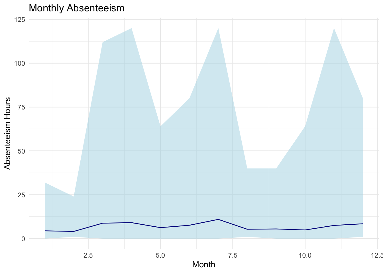
The code in above is used to create a visualization of the monthly_absenteeism_summary data using the ggplot2 package. The plot displays the average absenteeism hours for each month, with a shaded ribbon indicating the range between the maximum and minimum absenteeism hours.
The base layer of the plot is created with the ggplot() function. Within it, the dataset monthly_absenteeism_summary is specified, and aesthetic mappings are defined using the aes() function. This sets the Month.of.absence as the x-axis and the avg_absences (average absenteeism hours) as the y-axis. Atop this base, a ribbon is added using the geom_ribbon() function, which visually illustrates the range of absenteeism for each month. The minimum and maximum bounds of the ribbon are determined by the min_absences and max_absences columns, respectively. This ribbon is filled with a light blue color (fill="lightblue") and has a semi-transparent appearance due to the alpha=0.5 setting. Following the ribbon, a line is overlaid using the geom_line() function, which represents the average absenteeism hours for each month. This line is set to be dark blue in color. For better clarity, labels are then added to the plot using the labs() function, with the main title being “Monthly Absenteeism”, the x-axis labeled as “Month”, and the y-axis labeled as “Absenteeism Hours”. Finally, to give the plot a clean and minimalistic look, the theme_minimal() function is applied, which removes unnecessary gridlines and background colors.
This chart provides a visual representation of the monthly absenteeism trend with a clear view of the variation (range) in absenteeism for each month. The line indicates the average absenteeism, while the shaded ribbon shows the range between the maximum and minimum absenteeism values. This plot looks a bit weird, so lets check for outliers.
Step 5: Boxplot of Absenteeism Hours by Month
A boxplot is a great way to visualize the distribution of absenteeism hours for each month. Using the ggplot2 package, we’ll create a boxplot to visualize the distribution of absenteeism hours for each month:
ggplot(absenteeism_data, aes(x=factor(Month.of.absence), y=Absenteeism.time.in.hours)) +
  geom_boxplot(outlier.color="red", outlier.shape=16) +
  labs(title="Boxplot of Monthly Absenteeism Hours", x="Month", y="Absenteeism Hours") +
  theme_minimal()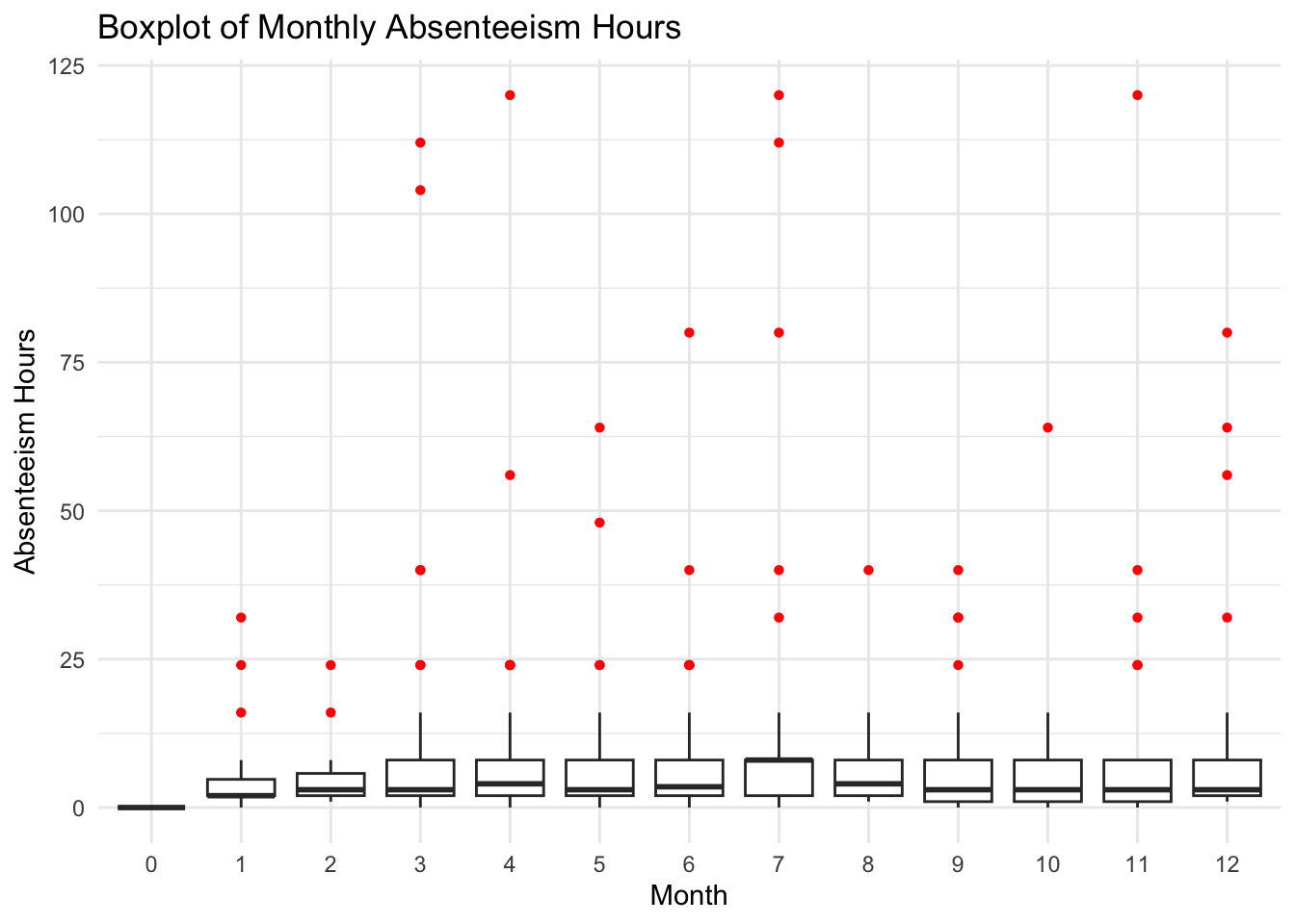
In this boxplot, the central line in each box represents the median absenteeism hours for the month, the edges of the box are the first and third quartiles, and the whiskers extend to the highest and lowest values within a reasonable range. Points outside the whiskers are outliers and are plotted in red. We can see there are a number of outliers.
Step 6: Visualization of Monthly Absenteeism without Outliers
In step 5 we see a lot of outliers. We can use the Tukey method to identifies outliers as values that fall outside of the whiskers in a box plot. Specifically, values below \(Q1 - 1.5 \times IQR\) or above \(Q3 + 1.5 \times IQR\) are considered outliers, where \(Q1\) is the first quartile, \(Q3\) is the third quartile, and \(IQR\) is the interquartile range (\(Q3 - Q1\)).
First, let’s identify and remove the outliers using the Tukey method:
# Calculate the IQR for Absenteeism.time.in.hours for each month
iqr_data <- absenteeism_data %>%
  filter(Month.of.absence!=0) %>%
  group_by(Month.of.absence) %>%
  summarise(Q1 = quantile(Absenteeism.time.in.hours, 0.25),
            Q3 = quantile(Absenteeism.time.in.hours, 0.75)) %>%
  mutate(IQR = Q3 - Q1,
         Lower_Bound = Q1 - 1.5*IQR,
         Upper_Bound = Q3 + 1.5*IQR)
In the code above, we calculate the interquartile range (IQR) of absenteeism hours for each month. The IQR is a measure of statistical spread and is calculated as the difference between the third (Q3) and first quartiles (Q1). It gives us insight into the middle 50% of the data, filtering out potential outliers.
Initially, the absenteeism_data is filtered to remove any entries with a month value of ‘0’, ensuring we’re only working with genuine monthly data. After this preliminary step, the data is grouped by Month.of.absence, allowing subsequent calculations to be specific to each individual month.
Using the summarise() function, the first (Q1) and third quartiles (Q3) of absenteeism hours are computed for each month. These quartiles give us an understanding of where 25% and 75% of the data lie, respectively.
The subsequent mutate() function then computes the IQR by subtracting Q1 from Q3. With the IQR in hand, we can then determine the lower and upper bounds for potential outliers using the common criterion: any data point lying below \(Q1 - 1.5 \times IQR\) or above \(Q3 + 1.5 \times IQR\) can be considered an outlier. These boundaries, labeled as Lower_Bound and Upper_Bound, are computed for each month and will be instrumental in filtering out extreme values in any subsequent analysis or visualization.
# Join the iqr_data with absenteeism_data and filter out outliers
filtered_data <- absenteeism_data %>%
  left_join(iqr_data, by = "Month.of.absence") %>%
  filter(Absenteeism.time.in.hours >= Lower_Bound & Absenteeism.time.in.hours <= Upper_Bound) %>%
  select(-c(Q1, Q3, IQR, Lower_Bound, Upper_Bound))
In the code above, the primary objective is to refine the absenteeism_data by eliminating data points deemed as outliers. To achieve this, the dataset iqr_data, which contains previously computed metrics such as the IQR and the boundaries for outlier identification (Lower_Bound and Upper_Bound) for each month, is merged with the primary absenteeism_data. This merge is executed through the left_join() function, with the joining condition specified by the Month.of.absence attribute.
Once the data is integrated, the filter() function is deployed to retain only those entries where the absenteeism hours fall within the established non-outlier range — that is, values greater than or equal to the Lower_Bound and less than or equal to the Upper_Bound for their respective months.
In the final step, the select() function is employed to remove superfluous columns related to the outlier computation process (Q1, Q3, IQR, Lower_Bound, and Upper_Bound) from the resultant dataset. This results in a cleaned dataset, designated as filtered_data, purged of outliers and streamlined for further analysis.
# Now, let's summarize the data for each month after removing outliers
monthly_absenteeism_summary_no_outliers <- filtered_data %>%
  group_by(Month.of.absence) %>%
  summarise(
    avg_absences = mean(Absenteeism.time.in.hours),
    max_absences = max(Absenteeism.time.in.hours),
    min_absences = min(Absenteeism.time.in.hours)
  )
Following the outlier removal, the next step taken in the code above is to generate a summarized view of the absenteeism hours on a monthly basis using the refined filtered_data. This summarization process groups the data by the Month.of.absence variable, ensuring that the subsequent metrics are computed for each individual month. Within each month grouping, three key metrics are calculated:
avg_absences: This captures the average absenteeism time, computed using the mean function on theAbsenteeism.time.in.hoursattribute.max_absences: This identifies the highest recorded absenteeism time within the month.min_absences: Contrarily, this determines the lowest recorded absenteeism time for the month.
The resultant dataset, named monthly_absenteeism_summary_no_outliers, presents a concise and clear depiction of absenteeism trends for each month, devoid of the influence of any extreme or anomalous values. This dataset can serve as a foundation for subsequent analytical endeavors or visual representations that aim to offer insights into employee absenteeism patterns.
# Visualization of Monthly Absenteeism without Outliers
ggplot(monthly_absenteeism_summary_no_outliers, aes(x=Month.of.absence, y=avg_absences)) +
  geom_ribbon(aes(ymin=min_absences, ymax=max_absences), fill="lightblue", alpha=0.5) +
  geom_line(color="darkblue") +
  labs(title="Monthly Absenteeism (Without Outliers)", x="Month", y="Absenteeism Hours") +
  theme_minimal()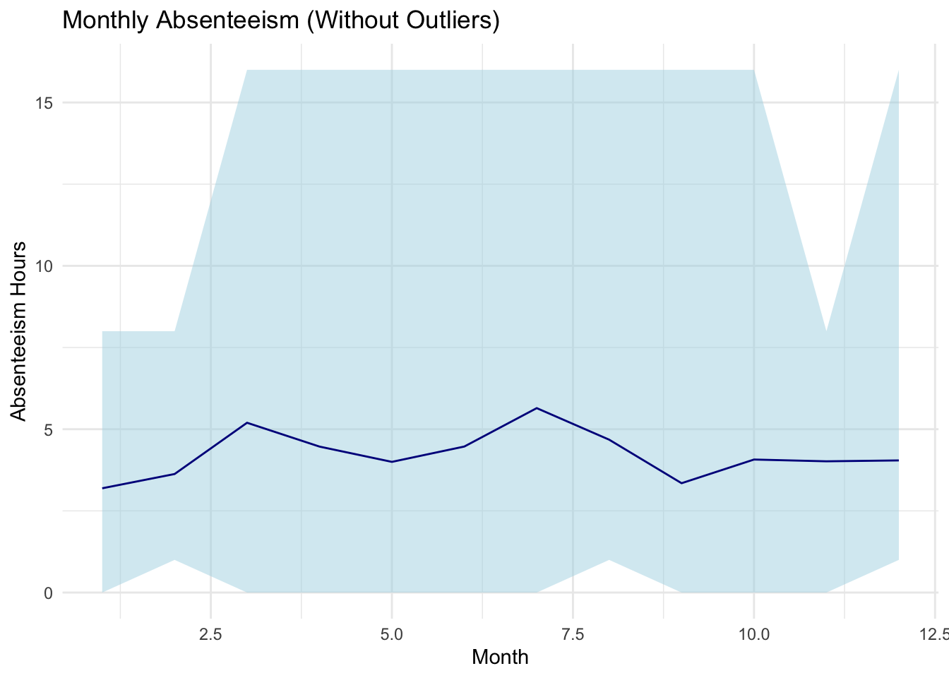
In the presented code, a visual representation is crafted to depict monthly absenteeism data, specifically after the removal of identified outliers. Utilizing the ggplot2 package, the code plots the average absenteeism hours per month from the dataset monthly_absenteeism_summary_no_outliers.
The foundation of the visualization is established using the ggplot() function, with the x-axis set to represent the Month.of.absence and the y-axis designated for the avg_absences, which denotes the average absenteeism hours.
A distinguishing feature of this plot is the incorporation of a shaded ribbon, introduced via the geom_ribbon() function. This ribbon provides a visual range for absenteeism hours, with its upper and lower bounds determined by the max_absences and min_absences, respectively. The light blue shade (fill="lightblue") of the ribbon, coupled with a semi-transparency setting (alpha=0.5), offers a subtle backdrop that accentuates the data’s spread for each month.
Overlaying this ribbon, a line graph is constructed using the geom_line() function, delineating the trend of average absenteeism across the months. The line’s dark blue hue (color="darkblue") ensures it remains distinct and prominent against the ribbon.
For enhanced clarity and context, the plot is adorned with labels via the labs() function. It bears the title “Monthly Absenteeism (Without Outliers)”, and both axes are appropriately labeled to signify “Month” and “Absenteeism Hours”.
Concluding the visualization’s aesthetics is the application of the theme_minimal(), bestowing the plot with a clean and clutter-free appearance. This graphical representation, in essence, offers stakeholders a lucid perspective on the month-wise absenteeism patterns, sans the distortion from outliers.
With in this step, outliers identified using the Tukey method have been removed before calculating the monthly summaries and visualizing the data. The resulting visualization provides an overview of absenteeism patterns without the influence of extreme values.
4.8 Summary
- The chapter covered the basics of working with R, including commands and calculations, functions, packages, comments, variables, data frames, lists, and formulas.
- Commands and calculations involve typing commands in the R console, performing arithmetic operations, and storing numeric values as variables.
- Functions play a crucial role in performing calculations and streamlining workflows, allowing for code modularity and reusability.
- Packages expand the functionality of R, and installing and loading packages is essential for accessing additional tools and capabilities.
- Comments provide annotations and explanations within code, improving code readability and maintainability.
- Variables in R can store different types of data, such as numbers, text, and logical values. Vectors are used to store multiple values of the same data type.
- Data frames are fundamental data structures in R for storing and manipulating tabular data.
- Lists are versatile structures in R that can hold elements of different types, providing flexibility and nesting capabilities.
- Formulas in R are used to specify mathematical relationships or statistical models, offering concise and expressive representations of variables’ relationships.
- Programming concepts like writing scripts, using loops for repetitive tasks, employing conditional statements for decision-making, and creating functions for modular code organization were introduced.
- Understanding these concepts provides a strong foundation for further exploration and proficiency in R programming and data analysis.
Martiniano, Andrea and Ferreira, Ricardo. (2018). Absenteeism at work. UCI Machine Learning Repository. https://doi.org/10.24432/C5X882.↩︎