3 Getting Started with R, RStudio and Posit.Cloud

PRELIMINARY AND INCOMPLETE

We begin with an introduction to R, a leading language for statistical computing, alongside RStudio, its essential integrated development environment (IDE). RStudio enhances R’s functionality by simplifying data analysis, visualization, and modeling, making these processes more accessible and efficient for users. We will cover the basics of R programming, including functions, variables, data frames, and more. Additionally, we will delve into essential programming concepts such as scripting, using loops, and creating functions. The learning objectives are designed to help you master the core functionalities of R, navigate and utilize RStudio effectively, extend R’s capabilities through the use of packages, manage complex data analyses using R’s various data structures, and develop robust data manipulation and analysis techniques.

Our adoption of a coding approach to business intelligence (BI) tools is designed to reveal the intricate details of analytical processes. This method not only demystifies underlying operations but also equips professionals with versatile skills applicable across various technologies. It fosters independence in data analysis and allows for deeper, more insightful engagements with data, ensuring that you gain a comprehensive understanding of both the tools and the theories behind them.

3.1 Chapter Goals

Upon concluding this chapter, readers will be equipped with the skills to:

Understand the fundamentals of R programming, including key functions, variables, and data structures, and how to utilize Posit.Cloud for web-based access to RStudio.
Navigate and utilize the RStudio Integrated Development Environment (IDE), including writing and executing R scripts, and employing loops and conditional statements for data manipulation.
Extend R’s functionality through packages, understanding their installation, management, and application within various data analysis projects.
Manipulate and analyze data using R’s core data structures such as vectors, data frames, and lists, applying functions and formulas for statistical analysis.
Develop and execute efficient R programming practices, including creating reusable functions, managing workspace, and effectively documenting code through comments for better readability and maintenance.

3.2 What is Posit.Cloud

Posit.Cloud is an innovative web service designed to offer a browser-based experience that closely emulates RStudio, a popular integrated development environment (IDE) for R programming. This programming language, R, is widely utilized for statistical computing and creating graphics. Posit.Cloud can be accessed via https://posit.cloud/.

RStudio, which Posit Cloud models, is typically available in two formats. The first is RStudio Desktop, an application run directly from a user’s computer. The second is RStudio Server, which operates from a remote server and allows users to access RStudio through a web browser. RStudio Server is the basis for Posit.Cloud.

Posit Cloud primarily targets educational settings, providing a useful tool for faculty and students involved in coursework. The service isn’t designed for individual use or extensive research purposes; for these applications, a standalone installation of RStudio on a local system is usually more appropriate.

Posit Cloud provides extensive documentation to assist users with the platform, accessible directly from the Posit Cloud website (https://posit.cloud/learn/guide). This resource, along with other support channels, ensures users can readily find the information they need to maximize their use of the service.

Posit Cloud offers four distinct subscription plans for users:

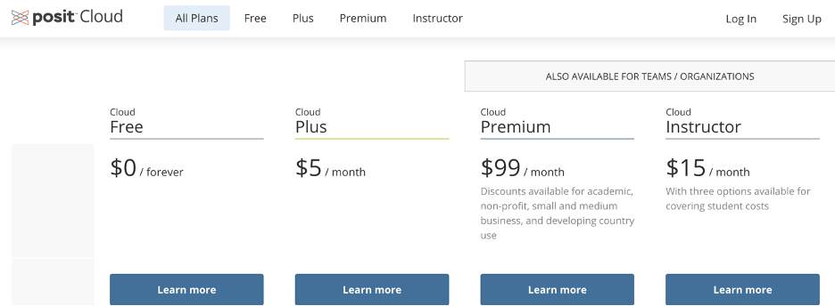
Cloud Free: This is a forever free plan. It includes access to 1 shared space (with member & project limits), 50 projects, 25 compute hours per month, a maximum of 1 GB RAM and 1 CPU, 1 hour max execution time, and 5 data connections. Concurrently, you can run up to 3 projects. However, this plan does not include online support, beta features access, or Single Sign-On (SSO) via SAML.

Cloud Plus: Priced at $5 per month, this plan also provides access to 1 shared space and 50 projects but includes 75 compute hours per month (with additional hours available at 10 cents per hour). The rest of the parameters are similar to the Cloud Free plan.

Cloud Premium: This plan is priced at $99 per month and offers unlimited shared spaces and projects. It comes with 200 compute hours included per month (additional hours are available at 10 cents per hour), 16 GB max RAM, 4 CPUs, 48 hours max execution time, and 30 data connections. Unlimited concurrent projects are allowed. It also includes online support, beta features access, and SSO via SAML for teams/organizations.

Cloud Instructor: Costing $15 per month, this plan is tailored for educators and offers similar specifications to the Cloud Premium plan but includes 300 compute hours per month. There are three options available for covering student costs, with unlimited hours with a fixed price per user plan also available.

This book will assume that the instructor has the Cloud Instructor plan; thus, the student will only need the Cloud Free plan.

3.3 Getting Ready for Class

If you are using Posit Cloud in a class where your instructor has a Cloud Instructor Posit Cloud account, you should get your Posit Cloud account setup. This process involves joining your class workgroup on the platform, enabling seamless collaboration and engagement with your classmates and instructor. This book is written with the assumption that your course instructor is using a Cloud Instructor Posit Cloud account. As such, your ideal starting point as a student would be to secure a Cloud Free plan. This plan provides the necessary features to participate in the class effectively, without any financial commitment. So, get started by setting up your account, join your class workgroup, and embark on your learning journey with Posit Cloud.

Step 1. Create an Account

Setting up a Posit.Cloud account on the Cloud Free plan is straightforward. Here are the steps:

Navigate to the Posit Cloud Free plan sign-up page by clicking on the following link: https://posit.cloud/plans/free.
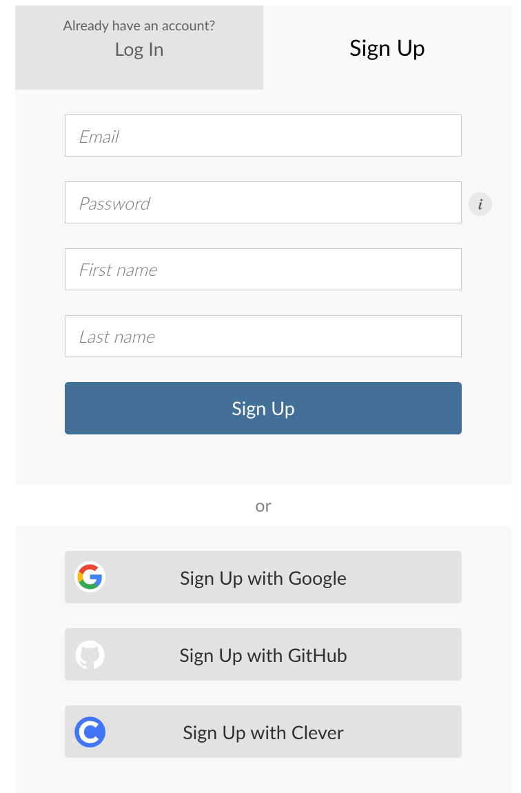
Once on the page, you’ll be prompted to fill out an account form.
When entering your email address, it’s recommended that you use your school email. This will make it easier to join your class workgroup later on, as your school email will likely be the identifier used to add you to the group.
After you’ve filled out the form with the necessary information, go ahead and submit it. You may be asked to verify your email address. If so, check your email (the one you just used to sign up) for a verification message from Posit Cloud. Follow the instructions in that email to verify your account.

Remember, it’s important to keep your login information secure, and make sure you’re the only one with access to your account to maintain your privacy and the integrity of your work.

3.3.1 Step 2. Join the Class Workspace

Posit.Cloud provides an innovative platform for organizing your projects into workspaces. One of the key features of workspaces is their shareability - a great tool for collaborative work! If your instructor is on a Cloud Instructor plan, they have the ability to share a class workspace with you. This means you gain access to all resources provided under the Cloud Instructor plan. Detailed instructions on how to join these class workspaces will be provided by your instructor.

3.4 Tour of RStudio

RStudio is an Integrated Development Environment (IDE) for R, a programming language for statistical computing and graphics. This section provides an overview of RStudio’s interface and basic functionality.

3.4.1 RStudio Layout

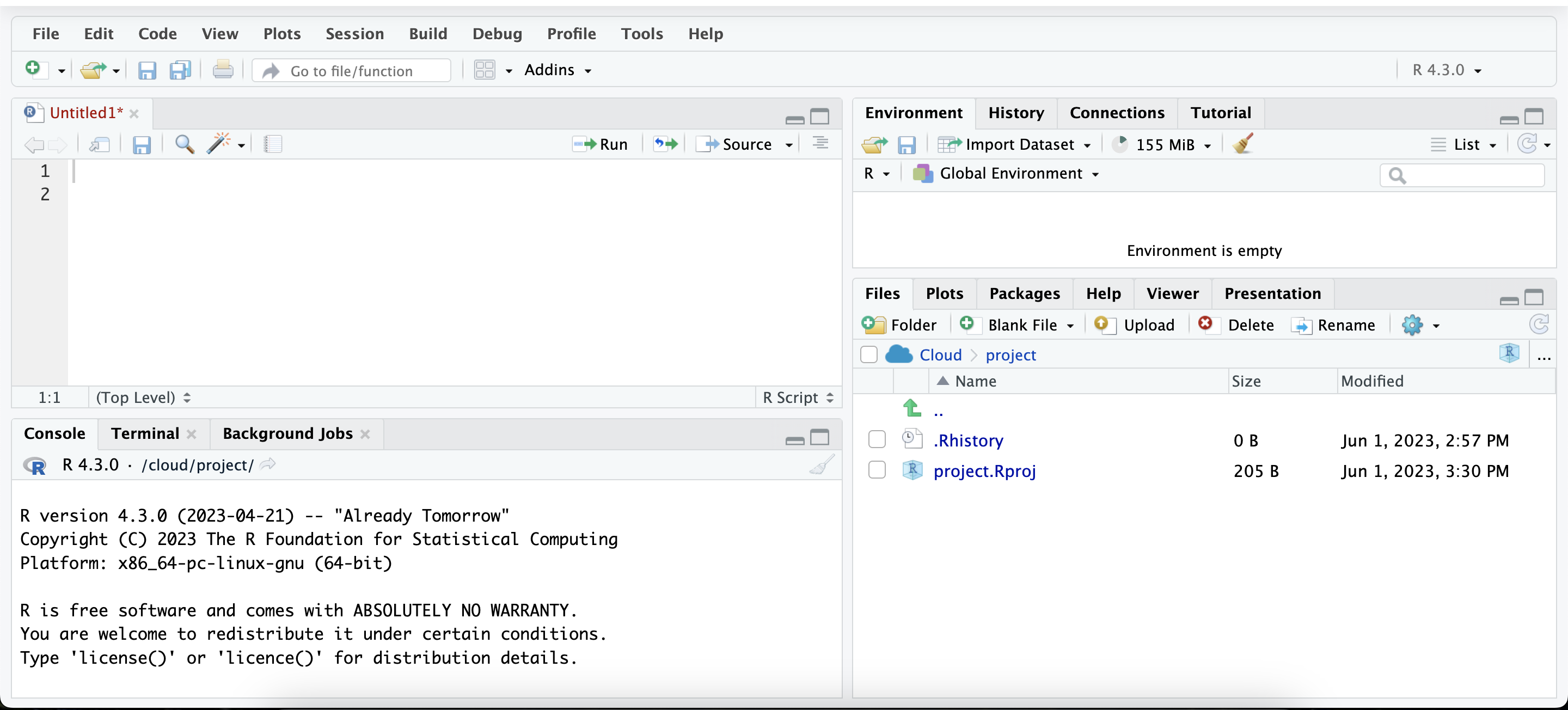
RStudio’s interface is divided into four main panels: the Source Panel, the Console Panel, the Environment/History Panel, and the Files/Plots/Packages/Help Panel.

3.4.1.1 Source Panel

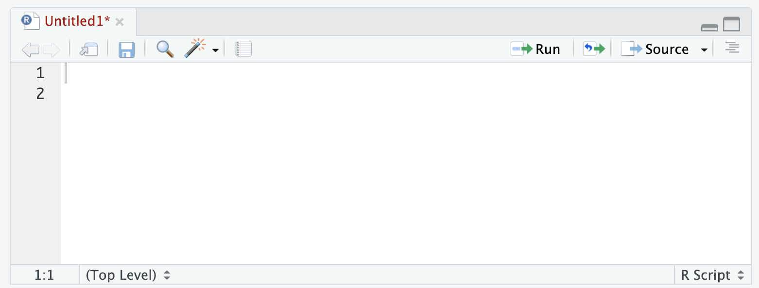
The top-left panel is the Source Panel, where R scripts, functions, and commands are written. New R scripts can be created via the menu options: File -> New File -> R Script.

3.4.1.2 Console Panel

Below the Source Panel is the Console Panel, where R code is executed. Any command executed in the script or typed directly into the console will appear here along with its output.

3.4.1.3 Environment/History Panel

The top-right panel is the Environment/History Panel. The Environment tab displays all variables, data frames, and other objects in the current workspace. The History tab keeps a record of command history.

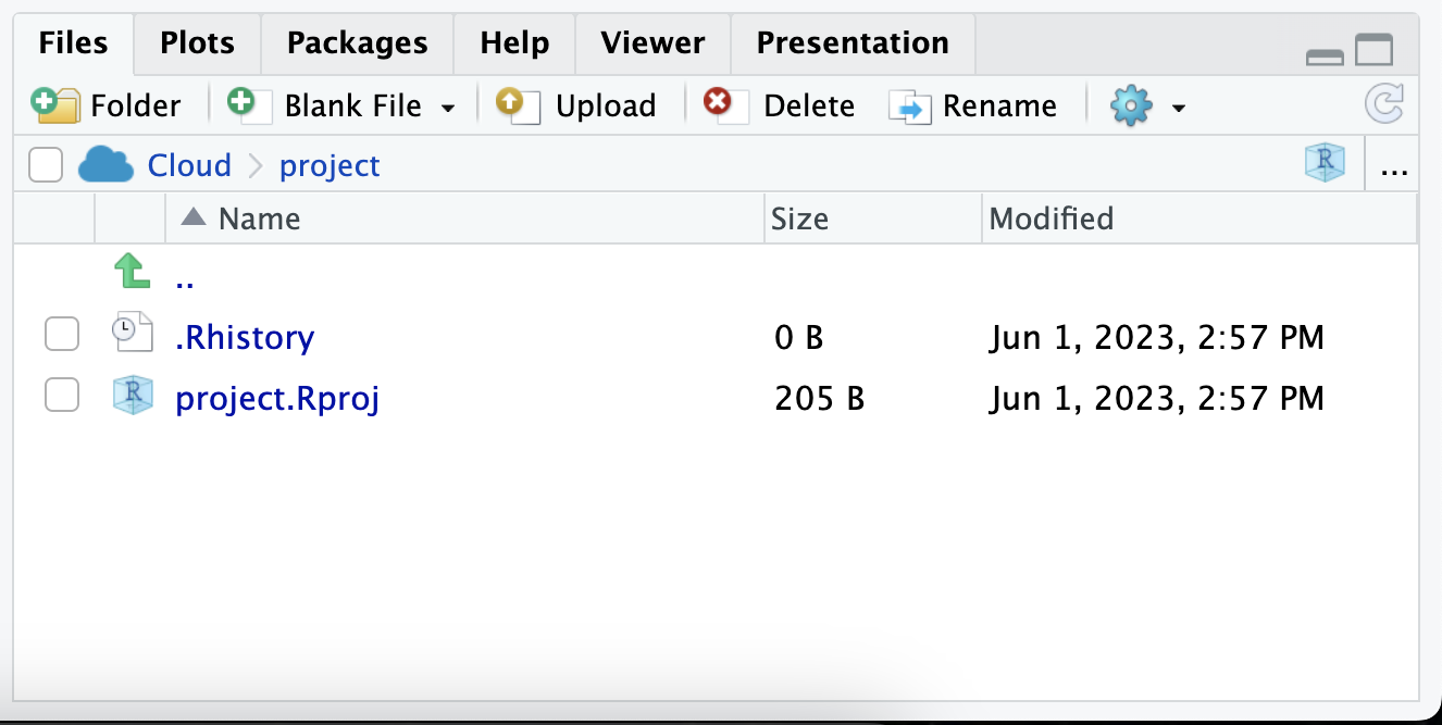
3.4.1.4 Files/Plots/Packages/Help Panel

The bottom-right panel is the Files/Plots/Packages/Help Panel. This panel provides access to files, any plots generated, R packages, and R’s help documentation.

3.4.2 Writing and Running R Code

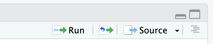
R scripts can be written in the Source Panel and executed in a few ways. To run the current line or selected lines, use Ctrl+Enter (or Cmd+Enter on a Mac) or click the “Run” button in the toolbar. To run the entire script, use the Source button in the toolbar.

3.4.3 Getting Help

RStudio provides comprehensive help documentation for R functions and packages. By using the ?functionName command, detailed help for any function can be accessed.

3.5 Commands and Calculations

In this section, we will explore interacting with the R programming environment, performing simple calculations, and storing numeric values as variables.

3.5.1 Typing Commands at the R Console

R is an interactive language that lets you type commands directly into its console. When you type a command at the R prompt and press “Enter”, R immediately provides the output. For instance, if you use the print() function as shown below, R will return Hello, World! in the console.

print("Hello, World!")

[1] "Hello, World!"

3.5.2 Doing Simple Calculations with R

R serves as both a programming language and a powerful calculator. You can perform basic arithmetic operations such as addition, subtraction, multiplication, division, and exponentiation. For instance, when you type 3 * 5 in the R console, as shown below, you will get 15 - the product of 3 and 5.

3 * 5

[1] 15

3.5.3 Storing a Number As a Variable

R enables you to store a numeric value as a variable for later use. This is accomplished using the assignment operator <-. For example, x <- 10 assigns the value 10 to the variable x. Once a value is stored as a variable, you can use it in future calculations. For instance, if you type x * 2 after assigning 10 to x, as shown below, R will return 20. This functionality is especially useful for performing complex operations and managing large datasets.

x <- 10
x * 2

[1] 20

3.6 Functions

Functions are an essential part of any programming language, including R. They allow you to encapsulate a set of instructions into a reusable block of code. This not only promotes code organization but also makes your programs more modular and easier to maintain. In this section, we will explore the concept of functions in R and how they can be used to perform calculations and streamline your workflow.

3.6.1 Using Functions to Do Calculations

One of the primary use cases of functions in R is to perform calculations. Instead of writing the same set of instructions repeatedly, you can use built-in functions to perform common calculations. In this example, we will use the mean() and sd() functions to calculate the mean and standard deviation of a variable in the mtcars dataset.

# Load the mtcars dataset
data(mtcars)

# Calculate the mean of the mpg variable
mpg_mean <- mean(mtcars$mpg)
print(mpg_mean)

[1] 20.09062

# Calculate the standard deviation of the mpg variable
mpg_sd <- sd(mtcars$mpg)
print(mpg_sd)

[1] 6.026948

In the above code chunk, we first load the mtcars dataset using the data() function. Then, we use the mean() function to calculate the mean of the mpg variable in the mtcars dataset. The mean() function takes a numeric vector as input and returns the arithmetic mean. We store the calculated mean in the variable mpg_mean and print it to the console using the print() function. Note that in the code chunk above, the lines that begin with # are comments. Comments are ignored by R.

Similarly, we use the sd() function to calculate the standard deviation of the mpg variable. The sd() function also takes a numeric vector as input and returns the standard deviation. We store the calculated standard deviation in the variable mpg_sd and print it to the console.

By using these functions, you can easily compute descriptive statistics for any variable in the mtcars dataset or any other dataset in R. The mean() function calculates the arithmetic mean, while the sd() function calculates the standard deviation.

3.6.2 Letting RStudio Help You with Your Commands

RStudio is an integrated development environment (IDE) that provides numerous features to assist you in writing and running R code efficiently. One of these features is the Code Completion functionality, which can save you time by suggesting completions for function names, arguments, and even file paths.

To use the Code Completion feature, simply start typing a function name or an object name in the RStudio editor and press the Tab key. RStudio will display a list of suggestions based on what you have typed so far. You can navigate through the suggestions using the arrow keys and press Enter to select a suggestion.

Additionally, RStudio provides a feature called Argument Help, which displays a pop-up window with detailed information about a function’s arguments and their usage. To access the Argument Help, type the function name followed by an opening parenthesis and press Tab. The pop-up window will appear, showing the function’s arguments, their data types, and a brief description.

Using these features in RStudio can significantly improve your productivity by providing suggestions and information about functions and their arguments as you write your code.

3.6.3 Basic and Commonly Used Functions in R

Here is a list of some basic and commonly used functions in R:

print(): Prints the specified object to the console.
sum(): Calculates the sum of a numeric vector.
length(): Returns the number of elements in an object.
head(): Displays the first few rows of a data frame or a vector.
tail(): Displays the last few rows of a data frame or a vector.
str(): Displays the structure of an object, showing its data type and dimensions.
subset(): Subsets a data frame based on specified conditions.
plot(): Creates a basic plot or a graphical visualization of data.
read.csv(): Reads a CSV file and imports its contents into a data frame.
write.csv(): Writes a data frame to a CSV file.
max(): Returns the maximum value in a vector.
min(): Returns the minimum value in a vector.
unique(): Returns the unique values in a vector or a data frame column.
table(): Creates a frequency table for categorical variables.
aggregate(): Applies a function to subsets of a data frame, based on one or more variables.

These functions represent just a small fraction of the vast collection of functions available in R. They serve various purposes and can be combined to perform complex data manipulation, analysis, and visualization tasks.

3.7 Vectors and Other Variables

Variables in R can hold various types of data, such as numbers, text, or logical values. One of the fundamental data structures in R is a vector, which allows you to store multiple values of the same data type in a single object. Note that unlike mathematics, in R, a vector is simply an ordered collection of elements of the same data type. In mathematics, a vector is a list of numbers.

3.7.1 Storing Many Numbers as a Vector

To store multiple numeric values in a vector, you can use the c() function, which stands for “combine” or “concatenate.” The c() function allows you to create a vector by combining individual elements. Here’s an example:

# Store a vector of numbers
numbers <- c(10, 20, 30, 40, 50)
print(numbers)

[1] 10 20 30 40 50

In the above code chunk, we create a vector called numbers using the c() function. The vector contains the values 10, 20, 30, 40, and 50. We then print the vector using the print() function, which displays the vector’s contents to the console.

3.7.2 Storing Text Data

In addition to storing numeric values, vectors in R can also store text data. Text data is referred to as character data in R. To create a vector of text values, you can enclose the values in quotes, either single (') or double ("). Here’s an example:

# Store a vector of names
names <- c("Alice", "Bob", "Charlie", "David")
print(names)

[1] "Alice"   "Bob"     "Charlie" "David"

In the above code chunk, we create a vector called names using the c() function. The vector contains the names “Alice”, “Bob”, “Charlie”, and “David”. We then print the vector to the console.

3.7.3 Storing “True or False” Data

In R, logical values (i.e., “true” or “false”) can be stored in vectors as well. The TRUE and FALSE constants are used to represent logical values. Here’s an example:

# Store a vector of logical values
logical_vector <- c(TRUE, FALSE, TRUE, TRUE)
print(logical_vector)

[1]  TRUE FALSE  TRUE  TRUE

In the above code chunk, we create a vector called logical_vector using the c() function. The vector contains the logical values TRUE, FALSE, TRUE, and TRUE. We then print the vector to the console. Note that TRUE, and FALSE and be abbreviate T and F, respectively.

3.7.4 Indexing Vectors

Indexing allows you to access and manipulate individual elements or subsets of a vector. In R, indexing starts at 1 (unlike some programming languages that start at 0). You can use square brackets ([]) to index vectors. Here are some examples:

# Accessing individual elements
numbers <- c(10, 20, 30, 40, 50)
print(numbers[1])  # Access the first element

[1] 10

# Accessing subsets
print(numbers[2:4])  # Access elements 2 to 4

[1] 20 30 40

# Modifying elements
numbers[3] <- 35

  # Change the value of the third element
print(numbers)

[1] 10 20 35 40 50

In the above code chunk, we create a vector called numbers using the c() function. We then demonstrate various indexing operations. The first example accesses the first element of the vector (10) by using numbers[1]. The second example accesses elements 2 to 4 of the vector (20, 30, 40) using numbers[2:4]. Finally, we modify the value of the third element of the vector from 30 to 35 using numbers[3] <- 35.

By understanding the concept of vectors and how to store different types of data, as well as indexing vectors, you can effectively work with collections of values in R.

3.8 Packages and Comments

In this section, we will explore the concept of packages in R and how they can enhance your coding experience. We will also discuss the importance of comments in your code and how they can improve its readability and maintainability.

3.8.1 Using Comments

Comments are lines of text in your code that are not executed as part of the program. They serve as annotations to explain the purpose or functionality of specific code sections. Comments are extremely useful for documenting your code, providing clarity to yourself and others who may read or work with your code.

# This is a comment in R. It is ignored by the program.

In the above code chunk, we use the # symbol to indicate a comment in R. Anything after the # symbol on the same line is treated as a comment and is not executed.

Comments can be used to:

Explain the purpose of functions or code blocks.
Provide instructions or guidance to other developers.
Temporarily disable or “comment out” lines of code for testing or debugging purposes.
Leave notes or reminders for future enhancements or improvements.

Using comments effectively can make your code more readable, maintainable, and understandable for yourself and others.

3.8.2 Installing and Loading Packages

Packages are collections of R functions, data, and documentation that extend the functionality of R. They are created and maintained by the R community and provide additional tools for various purposes, such as data manipulation, statistical analysis, plotting, and more.

To use a package in R, you need to install it first using the install.packages() function. Once installed, you can load the package into your R session using the library() or require() function.

# Install a package
install.packages("package_name")

# Load a package
library("package_name")

In the above code chunk, replace "package_name" with the actual name of the package you want to install or load. The install.packages() function downloads and installs the specified package from the comprehensive R Archive Network (CRAN). The library() function loads the installed package into your R session, making its functions and features available for use.

Packages greatly expand the capabilities of R and are essential for many data analysis tasks. They are designed to be modular, allowing you to choose and load only the packages you need for a specific project.

3.8.3 Managing the Workspace

The workspace in R refers to the current working environment where objects (variables, functions, datasets) are stored. Managing the workspace effectively is crucial for organizing and maintaining your code.

To view the objects in your workspace, you can use the ls() function. It lists all the objects currently stored in your workspace.

# List objects in the workspace
ls()

The rm() function is used to remove objects from the workspace.

# Remove an object from the workspace
rm(object_name)

Replace "object_name" with the name of the object you want to remove.

Managing the workspace allows you to keep your environment clean and avoid clutter. By removing unnecessary objects, you can free up memory and avoid potential conflicts or confusion in your code.

By understanding how to use comments effectively, installing and loading packages, and managing your workspace, you can enhance your coding experience in R and improve the organization and readability of your code.

3.9 Working with Data Frames, Lists, and Formulas

In this section, we will explore three important data structures in R: data frames, lists, and formulas. These structures provide flexible ways to work with and manipulate data in R.

3.9.1 Loading and Saving Data

Loading external data into R is a common task in data analysis. R provides various functions to read data from different file formats, such as CSV, Excel, or databases. Similarly, you can save data from R to these file formats.

# Load data from a CSV file
data <- read.csv("data.csv")

# Save data to a CSV file
write.csv(data, "output.csv")

In the above code chunk, the read.csv() function is used to load data from a CSV file named “data.csv” into a data frame called data. Conversely, the write.csv() function saves the data frame data to a new CSV file named “output.csv”. You can replace the file names and formats as needed.

3.9.2 Factors

In R, factors are used to represent categorical data. Factors are created using the factor() function and can have predefined levels.

# Create a factor
gender <- factor(c("Male", "Female", "Male", "Male"))
print(gender)

[1] Male   Female Male   Male  
Levels: Female Male

In the above code chunk, we create a factor called gender using the factor() function. The factor consists of the categories “Male”, “Female”, “Male”, and “Male”. When printed, the factor displays the levels and the corresponding categories.

Factors are useful for encoding categorical variables and conducting statistical analyses or modeling on such variables.

3.9.3 Data Frames

Data frames are a fundamental data structure in R that allow you to store and manipulate tabular data. A data frame is a collection of vectors, each representing a column, combined into a single object.

# Create a data frame
df <- data.frame(
  name = c("Alice", "Bob", "Charlie"),
  age = c(25, 30, 35),
  salary = c(50000, 60000, 70000)
)
print(df)

     name age salary
1   Alice  25  50000
2     Bob  30  60000
3 Charlie  35  70000

In the above code chunk, we create a data frame called df using the data.frame() function. The data frame consists of three columns: “name”, “age”, and “salary”. Each column is represented by a vector containing corresponding values. When printed, the data frame displays the tabular structure.

Data frames are commonly used for organizing and analyzing data, as they allow you to perform operations on entire columns or subsets of data.

3.9.4 Lists

Lists are another versatile data structure in R that can hold elements of different data types, including vectors, data frames, and even other lists. Lists are created using the list() function.

# Create a list
my_list <- list(
  name = "John",
  age = 30,
  hobbies = c("reading", "playing guitar"),
  address = data.frame(street = "123 Main St", city = "Anytown")
)
print(my_list)

$name
[1] "John"

$age
[1] 30

$hobbies
[1] "reading"        "playing guitar"

$address
       street    city
1 123 Main St Anytown

In the above code chunk, we create a list called my_list using the list() function. The list contains elements of different types, such as a character string, numeric value, vector, and a data frame. When printed, the list displays its elements and their respective values.

Lists are useful for organizing and managing complex data structures, as they can hold heterogeneous elements and allow for nested structures.

3.9.5 Formulas

Formulas are a unique feature in R that are used to specify mathematical relationships or statistical models. Formulas are created using the ~ symbol and are commonly used in functions such as regression models.

# Create a formula
my_formula <- mpg ~ cyl + disp
print(my_formula)

mpg ~ cyl + disp

In the above code chunk, we create a formula called my_formula using the ~ symbol. The formula specifies a relationship between the mpg variable and the cyl and disp variables. When printed, the formula displays the formula expression.

Formulas allow for concise and expressive representation of relationships between variables, making them particularly useful in statistical modeling and data analysis.

By understanding data frames, lists, and formulas, you can effectively organize and manipulate data in R, enabling you to perform various data analysis tasks and statistical modeling.

3.10 Programming in R

In this section, we will explore the basics of programming in R, including writing scripts, using loops, conditional statements, and writing functions.

3.10.1 Writing Scripts

Writing R scripts allows you to create a sequence of R commands that can be executed together. Scripts are particularly useful for automating tasks or organizing your code into reusable blocks. You can use any text editor or integrated development environment (IDE) to write R scripts.

# Example R script
# This script calculates the square of a number

# Define a function to calculate the square
square <- function(x) {
  return(x^2)
}

# Perform calculations
number <- 5
result <- square(number)
print(result)

[1] 25

In the above code, we have an example R script. We define a function called square() that calculates the square of a number. We then perform calculations by calling the square() function with a value of 5 and store the result in the result variable. Finally, we print the result to the console using the print() function.

Writing scripts allows you to organize and execute multiple commands in a systematic manner, making your code more readable and reusable.

3.10.2 Loops

Loops in R allow you to repeatedly execute a block of code. They are useful when you want to perform a task multiple times, iterating over a sequence of values or elements.

# Example of a for loop
for (i in 1:5) {
  print(i)
}

[1] 1
[1] 2
[1] 3
[1] 4
[1] 5

In the above code, we have an example of a for loop. It iterates over the sequence of numbers from 1 to 5 and prints each number to the console.

There are also other types of loops in R, such as while and repeat loops, which execute a block of code based on certain conditions or until a specific condition is met.

Loops are powerful tools for automating repetitive tasks and performing iterative operations.

3.10.3 Conditional Statements

Conditional statements allow you to control the flow of your code based on specific conditions. In R, the most common conditional statement is the if-else statement.

# Example of an if-else statement
x <- 10
if (x > 5) {
  print("x is greater than 5")
} else {
  print("x is less than or equal to 5")
}

[1] "x is greater than 5"

In the above code, we have an example of an if-else statement. It checks whether the value of x is greater than 5. If the condition is true, it prints the message “x is greater than 5”. Otherwise, it executes the code in the else block and prints “x is less than or equal to 5”.

Conditional statements allow your code to make decisions and execute different blocks of code based on specific conditions, providing flexibility and control.

3.10.4 Writing Functions

Functions in R allow you to encapsulate a set of instructions into a reusable block of code. They enable modular programming and help to organize and structure your code.

# Example of a function
calculate_average <- function(x, y) {
  avg <- (x + y) / 2
  return(avg)
}

# Call the function
result <- calculate_average(5, 7)
print(result)

[1] 6

In the above code, we define a function called calculate_average() that takes two arguments, x and y. The function calculates the average of the two values and returns the result. We then call the function with arguments 5 and 7 and store the result in the result variable. Finally, we print the result to the console.

Functions help modularize your code, making it easier to read, maintain, and reuse. They are essential for code organization and can improve the efficiency of your programming tasks.

By understanding the basics of programming in R, including writing scripts, using loops, conditional statements, and writing functions, you can harness the full power of R to solve complex problems and automate tasks.

3.11 Summary

The chapter covered the basics of working with R, including commands and calculations, functions, packages, comments, variables, data frames, lists, and formulas.
Commands and calculations involve typing commands in the R console, performing arithmetic operations, and storing numeric values as variables.
Functions play a crucial role in performing calculations and streamlining workflows, allowing for code modularity and reusability.
Packages expand the functionality of R, and installing and loading packages is essential for accessing additional tools and capabilities.
Comments provide annotations and explanations within code, improving code readability and maintainability.
Variables in R can store different types of data, such as numbers, text, and logical values. Vectors are used to store multiple values of the same data type.
Data frames are fundamental data structures in R for storing and manipulating tabular data.
Lists are versatile structures in R that can hold elements of different types, providing flexibility and nesting capabilities.
Formulas in R are used to specify mathematical relationships or statistical models, offering concise and expressive representations of variables’ relationships.
Programming concepts like writing scripts, using loops for repetitive tasks, employing conditional statements for decision-making, and creating functions for modular code organization were introduced.
Understanding these concepts provides a strong foundation for further exploration and proficiency in R programming and data analysis.