12 Case Study: Anomaly Detection
PRELIMINARY AND INCOMPLETE
Understanding the underlying patterns in employee behavior and identifying anomalies are essential for enhancing organizational efficiency and managing employee behavior effectively. Anomalies, or outliers, in data can often reveal significant, yet previously unnoticed, events or errors, such as data entry errors, fraud, or deviations in employee behavior. This chapter explores the application of anomaly detection techniques to the “Absenteeism at Work” dataset, a detailed compilation of information on employee absenteeism within a workplace. By leveraging sophisticated statistical methods, we aim to uncover unusual patterns and deepen our understanding of the factors driving employee absenteeism.
In this case study, we will examine three robust anomaly detection methods, each offering a distinct approach to identifying outliers:
Linear Regression Model with Examination of Residuals: We begin with a linear regression analysis to predict absenteeism hours based on various predictors such as the reason for absence, time of year, employee workload, and personal or family responsibilities. The residuals from this model—the differences between observed and predicted values—serve as a means to identify data points that significantly diverge from predicted patterns, suggesting potential anomalies.
K-Nearest Neighbors (k-NN): The k-NN method will be employed to detect anomalies by examining the local neighborhood of each data point. In this approach, an anomaly is considered as an observation that lies at an abnormal distance from its neighbors. By adjusting the parameters of the k-NN algorithm, such as the number of neighbors, we can effectively discern what constitutes normal and abnormal absenteeism behavior.
Random Forest: Random Forest, a powerful ensemble method, will be utilized to classify and detect outliers in the absenteeism data. By building multiple decision trees and observing their predictions about the normality or abnormality of data points, Random Forest offers a consensus approach that bolsters the reliability of anomaly detection.
12.1 Data Loading and Preparation
We begin our analysis by importing the “Absenteeism at Work” dataset, which is hosted online in CSV format. The R code snippet below loads the data into our R environment using a semicolon as the delimiter to ensure accurate column separation. This initial step is crucial as it prepares the dataset for detailed analysis and modeling to better understand patterns of absenteeism.
The head function allows us to preview the first few rows of the dataset, ensuring it is loaded correctly.
The next block of R code relabels the day and month columns to make them more interpretable. We use the lubridate package to convert numerical day and month values into more readable formats, using weekday and abbreviated month names.
We then narrow down the dataset to focus on specific attributes that are key for further analyses, effectively shaping our dataset to include variables that are most relevant.
Following this, we recode several categorical variables to enhance clarity and remove redundant variables. This includes recoding smoker and drinker status, and condensing the number of children and pets into more meaningful categories.
absenteeism <- absenteeism |>
  mutate(
    Social.smoker = ifelse(Social.smoker == 0, "Non-smoker", "Smoker"),
    Social.drinker = ifelse(Social.drinker == 0, "Non-drinker", "Social drinker"),
    Children = ifelse(Son == 0, "Non-parent", "Parent"),
    Pet = ifelse(Pet == 0, "No Pet(s)", "Pet(s)")
  ) |>
  select(-Son)
Next, the education variable is simplified into broader categories to facilitate easier analysis and interpretation.
Finally, we ensure all categorical variables are converted to factors for proper analysis. This step is important for statistical modeling and analyses that require categorical data to be explicitly declared.
After these transformations, a second head function call provides a snapshot of the updated dataset.
This refined dataset is now ready to be used in various methods of anomaly detection.
12.2 Identifying Anomalies Using Linear Regression
In a previous case study, we used linear regression to examine the variables driving absenteeism. Building on this foundation, we now shift our focus to the application of linear regression for anomaly detection. Unlike the previous scenarios where data might have been aggregated by specific categories such as employee groups, this section examines each individual absence.
The process begins by fitting a linear regression model to the dataset without aggregating by employee. After fitting the model, we proceed to identifying anomalies. This step involves pinpointing observations that significantly deviate from the model’s predictions, particularly those that surpass a predefined threshold of expected values.
Once these outliers are identified, the next phase involves a detailed examination of their characteristics. By scrutinizing these anomalies, we can gain insights into how occurrences differ from the norm, potentially uncovering underlying issues or exceptional cases within the dataset. This analysis not only deepens our understanding but also aids in refining our approach to managing absenteeism effectively.
12.2.1 Fitting a linear model
To analyze absenteeism, we begin by fitting a linear regression model. The response variable, the logarithm of absenteeism hours, is modeled as a function of all other variables in the dataset. Using a logarithmic transformation helps normalize the response variable’s distribution, a typical prerequisite for effective linear regression.
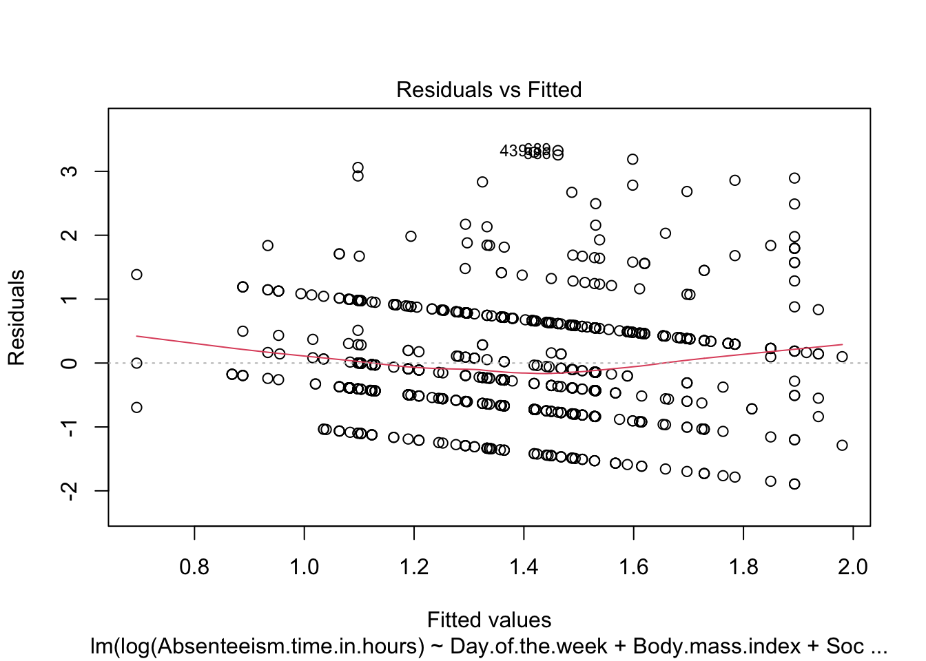
Next, we examine the model’s summary, which provides essential details such as coefficients, residuals, and other diagnostic metrics to evaluate the fit and effectiveness of the model. Understanding the influence of each predictor and the overall model quality is crucial.
MODEL INFO:
Observations: 696
Dependent Variable: log(Absenteeism.time.in.hours)
Type: OLS linear regression

MODEL FIT:
F(11,684) = 4.44, p = 0.00
R² = 0.07
Adj. R² = 0.05

Standard errors: OLS
--------------------------------------------------------
                             Est.   S.E.   t val.      p
------------------------- ------- ------ -------- ------
(Intercept)                  1.44   0.28     5.20   0.00
Day.of.the.weekSat           0.01   0.12     0.09   0.93
Day.of.the.weekThu           0.26   0.12     2.26   0.02
Day.of.the.weekTue           0.42   0.12     3.62   0.00
Day.of.the.weekWed           0.23   0.12     1.97   0.05
Body.mass.index             -0.02   0.01    -1.49   0.14
Age                         -0.00   0.01    -0.16   0.88
Social.smokerSmoker          0.09   0.16     0.57   0.57
Social.drinkerSocial         0.30   0.09     3.36   0.00
drinker
PetPet(s)                   -0.09   0.11    -0.86   0.39
ChildrenParent               0.30   0.10     2.90   0.00
CollegeHigh School          -0.09   0.11    -0.76   0.45
--------------------------------------------------------
We also generate diagnostic plots for the regression model. Specifically, plotting residuals against fitted values (specified by which = 1) is critical for assessing model assumptions such as non-linearity, identifying outliers, and checking for constant variance of residuals (homoscedasticity).

To optimize the model, a stepwise regression process is employed to either reduce or adjust the explanatory variables based on the Akaike Information Criterion (AIC). This stepwise adjustment helps in achieving a more parsimonious model that balances complexity with fit.
Following the model refinement through stepwise regression, the updated summary of the model is reviewed to note any changes and assess the overall fit with the adjusted set of variables.
MODEL INFO:
Observations: 696
Dependent Variable: log(Absenteeism.time.in.hours)
Type: OLS linear regression

MODEL FIT:
F(7,688) = 6.68, p = 0.00
R² = 0.06
Adj. R² = 0.05

Standard errors: OLS
-------------------------------------------------------
                            Est.   S.E.   t val.      p
------------------------ ------- ------ -------- ------
(Intercept)                 1.48   0.25     5.89   0.00
Day.of.the.weekSat          0.02   0.12     0.17   0.87
Day.of.the.weekThu          0.26   0.12     2.25   0.03
Day.of.the.weekTue          0.43   0.11     3.71   0.00
Day.of.the.weekWed          0.23   0.12     1.96   0.05
Body.mass.index            -0.02   0.01    -2.39   0.02
Social.drinkerSocial        0.30   0.08     3.93   0.00
drinker
ChildrenParent              0.23   0.07     3.23   0.00
-------------------------------------------------------
To confirm improvements in model assumptions, such as reduced patterns in residuals and enhanced homogeneity of variance, the diagnostic plot is revisited for the refined model.
The steps described complete a detailed examination and adjustment of the regression model, ensuring its suitability for detecting anomalies in absenteeism data.
12.2.2 Identify Anomalous Residuals
To detect anomalies in the absenteeism data, we first establish a threshold for the residuals from our linear regression model. Anomalies are identified based on the magnitude of the residuals, with larger residuals indicating greater deviations from the predicted model. We set the threshold at twice the standard deviation of the residuals, a common choice for outlier detection which typically captures the most extreme variations.
Next, we visualize these anomalous observations by plotting the residuals against the fitted values. This plot helps in visually identifying data points where the residuals exceed the established threshold. Points with residuals above this threshold are highlighted in red, distinguishing them from typical data points (shown in black).
To identify and visualize anomalous observations effectively, we use the following R code:
# Create a dataframe for plotting the residuals and their corresponding fitted values
plot_data <- data.frame(
  Fitted = anomaly.lm$fitted.values,
  Residuals = anomaly.lm$residuals
)

# Generate the plot of residuals versus fitted values
ggplot(plot_data, aes(x = Fitted, y = Residuals)) +
  geom_hline(yintercept = 0, linetype = "dashed", color = "grey") +
  geom_point(aes(color = Residuals > threshold)) +
  scale_color_manual(values = c("black", "red")) +
  labs(title = "Residual vs. Fitted Plot",
       x = "Fitted Values",
       y = "Residuals",
       color = "Threshold Exceeded") +
  theme_minimal()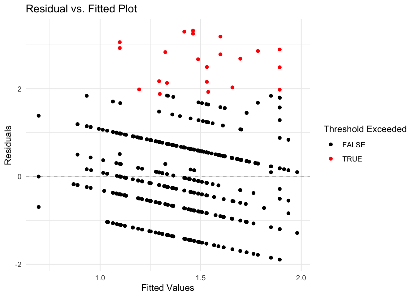
Breaking Down the Code
-
Data Frame Creation: A data frame
plot_datais created containing two columns:Fitted(model’s predicted values) andResiduals(differences between observed and predicted values). -
Residual Plot: Using
ggplot, the data frame is plotted withFittedvalues on the x-axis andResidualson the y-axis.- Horizontal Line: A horizontal dashed line at zero is added to visually separate positive and negative residuals, aiding in identifying patterns or bias in the residuals.
- Color Coding: Points are colored to distinguish normal residuals (black) from anomalies (red), based on whether residuals exceed the predefined threshold.
- Plot Aesthetics: Titles and labels are added to improve readability and understanding of the plot, and a minimalistic theme is applied for visual clarity.
This visualization is helpful for pinpointing unusual data points that may indicate anomalies, facilitating further investigation into specific cases of absenteeism.
12.2.3 Analysis of Anomalies Identifyed in a Dataset
Once anomalies are identified in a dataset, the next step is to conduct both descriptive and graphical analyses to compare anomalous and non-anomalous observations. This section covers how to perform these analyses using R, a statistical programming language, providing insights into the differences and implications of these observations in your dataset.
Helper Functions for Anomaly Detection
In the context of anomaly detection, two specific R functions, anomaly.boxplot and anomaly.barplot, have been designed to aid in the exploration and analysis of data by visualizing the distribution of numeric and categorical variables respectively against an anomaly indicator. These functions are essential for identifying and understanding patterns or outliers in different data types.
The anomaly.boxplot Function
The anomaly.boxplot function is crucial for analyzing numeric data. It begins by confirming the presence of an anomaly indicator within the dataset. Once validated, it identifies all numeric columns which are then subjected to further visual analysis. For each numeric column, the function generates a box plot, which segments the numeric values according to the categories of the anomaly indicator. This visualization allows for an easy comparison across categories, highlighting potential outliers or anomalies. Each box plot details the median, quartiles, and outliers, providing a clear statistical summary of the data. The plots are arranged in a grid with two columns, simplifying the comparison process and helping quickly spot any irregular patterns that may need deeper investigation.
anomaly.boxplot <- function(data, anomaly_indicator) {
  if (!anomaly_indicator %in% names(data)) {
    stop("Anomaly indicator column not found in the data frame.")
  }
  numeric_columns <- sapply(data, is.numeric)
  numeric_columns <- names(numeric_columns[numeric_columns])
  plot_list <- list()
  for (num_col in numeric_columns) {
    plot <- ggplot(data, aes_string(x = anomaly_indicator, y = num_col)) +
      geom_boxplot() +
      labs(title = paste(num_col),
           x = anomaly_indicator,
           y = num_col) +
      theme_minimal()
    plot_list[[num_col]] <- plot
  }
  plot_grid <- wrap_plots(plot_list, ncol = 2)
  print(plot_grid)
}
The anomaly.barplot Function
Conversely, the anomaly.barplot function is tailored for examining categorical data. It also starts by ensuring the anomaly indicator column is present in the dataset. It then identifies all categorical columns, filtering out the anomaly indicator if it is mistakenly categorized as such. For each identified categorical variable, the function computes the proportion of data falling into each category of the anomaly indicator and visualizes this information using bar plots. This setup provides a transparent visualization of how categorical data is distributed across different anomaly classifications, facilitating an easy assessment of how these variables interact with potential anomalies. The individual plots are organized into a two-column grid, enhancing the visual comparison across variables.
anomaly.barplot <- function(data, anomaly_indicator) {
  if (!anomaly_indicator %in% names(data)) {
    stop("Anomaly indicator column not found in the data frame.")
  }
  categorical_columns <-
    sapply(data, is.factor) | sapply(data, is.character)
  categorical_columns <-
    names(categorical_columns[categorical_columns])
  categorical_columns <-
    categorical_columns[categorical_columns != anomaly_indicator]
  plot_list <- list()
  for (cat_col in categorical_columns) {
    xtab <-
      xtabs(reformulate(c(cat_col, anomaly_indicator), response = NULL),
            data = data)
    xtab <- prop.table(xtab, margin = 2)
    xtab_df <- as.data.frame(as.table(xtab))
    colnames(xtab_df) <- c(cat_col, anomaly_indicator, "Freq")
    plot_list[[cat_col]] <-
      ggplot(xtab_df,
             aes_string(x = anomaly_indicator, y = "Freq", fill = cat_col)) +
      geom_bar(stat = "identity", position = "stack") +
      labs(
        title = paste(cat_col),
        x = "",
        y = "Proportion",
        fill = cat_col
      ) +
      theme_minimal() +
      guides(fill = guide_legend(title = NULL))
  }
  plot_grid <- wrap_plots(plot_list, ncol = 2)
  print(plot_grid)
}
These functions represent critical tools in the anomaly detection toolkit, each addressing different aspects of the data and providing comprehensive insights that are pivotal for effective anomaly detection.
Visualize analysis anomalies
To further analyze anomalies in the absenteeism data, we first create a modified version of the original dataset and store it in a new data frame named absenteeism.lm. In this data frame, we add a new column called IsAnomalous. This column categorizes each entry as TRUE if the corresponding residual from the linear regression model (stored in anomaly.lm$residuals) exceeds a predefined threshold, thereby labeling it as an anomaly. Here’s the R code for creating this enhanced data frame:
Next, we visualize the anomalies using box plots and bar plots to compare the distributions of numeric and categorical data, respectively, between anomalous and non-anomalous observations.
# Generate box plots for numeric data categorized by anomaly status
anomaly.boxplot(data = absenteeism.lm, anomaly_indicator = "IsAnomalous")
Warning: `aes_string()` was deprecated in ggplot2 3.0.0.
ℹ Please use tidy evaluation idioms with `aes()`.
ℹ See also `vignette("ggplot2-in-packages")` for more information.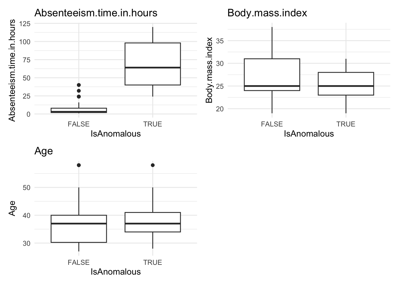
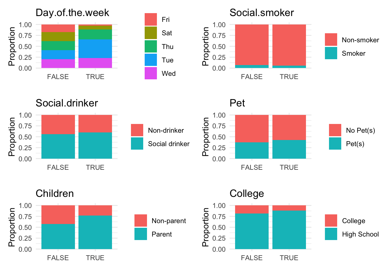
# Generate bar plots for categorical data categorized by anomaly status
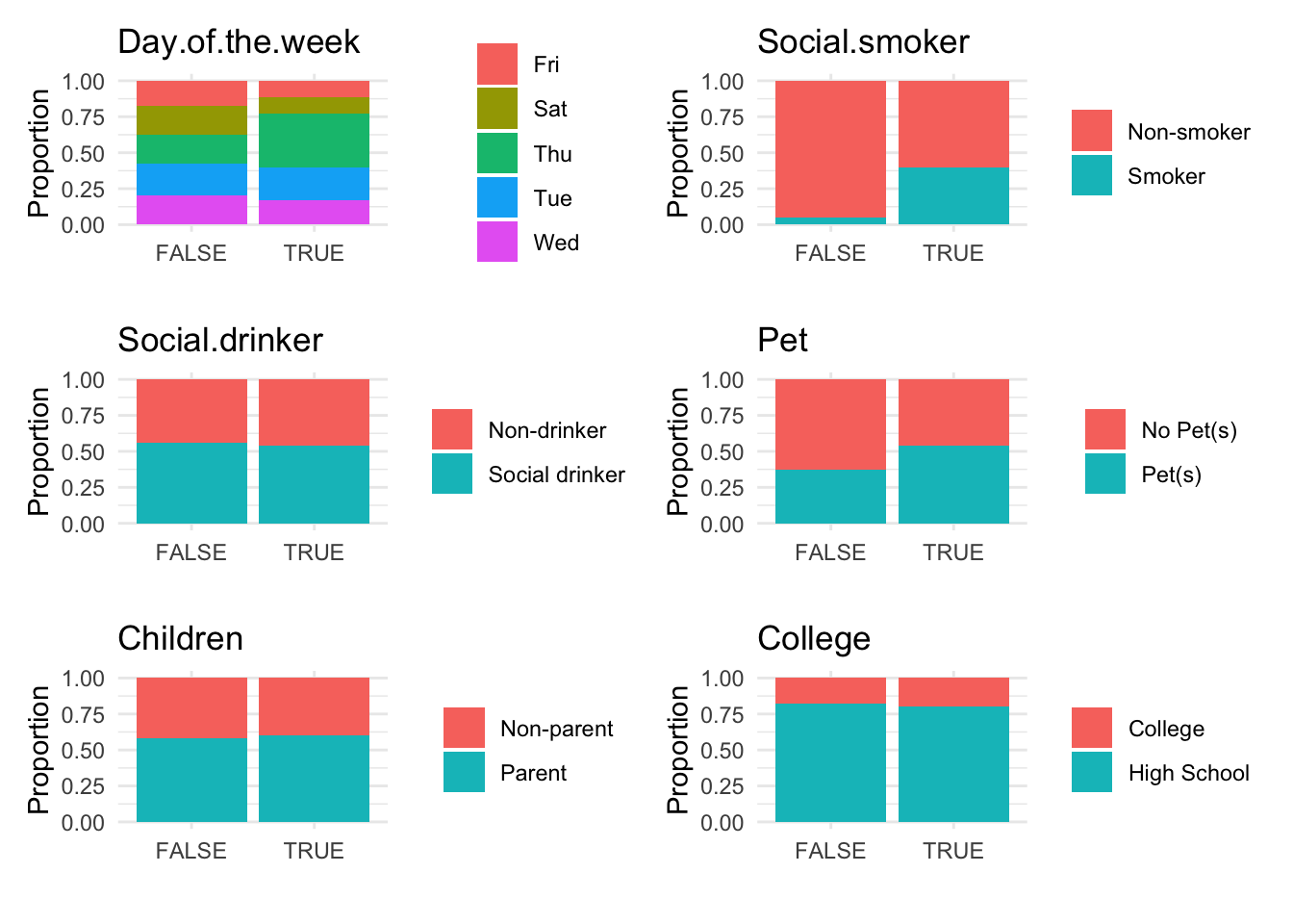
anomaly.barplot(data = absenteeism.lm, anomaly_indicator = "IsAnomalous")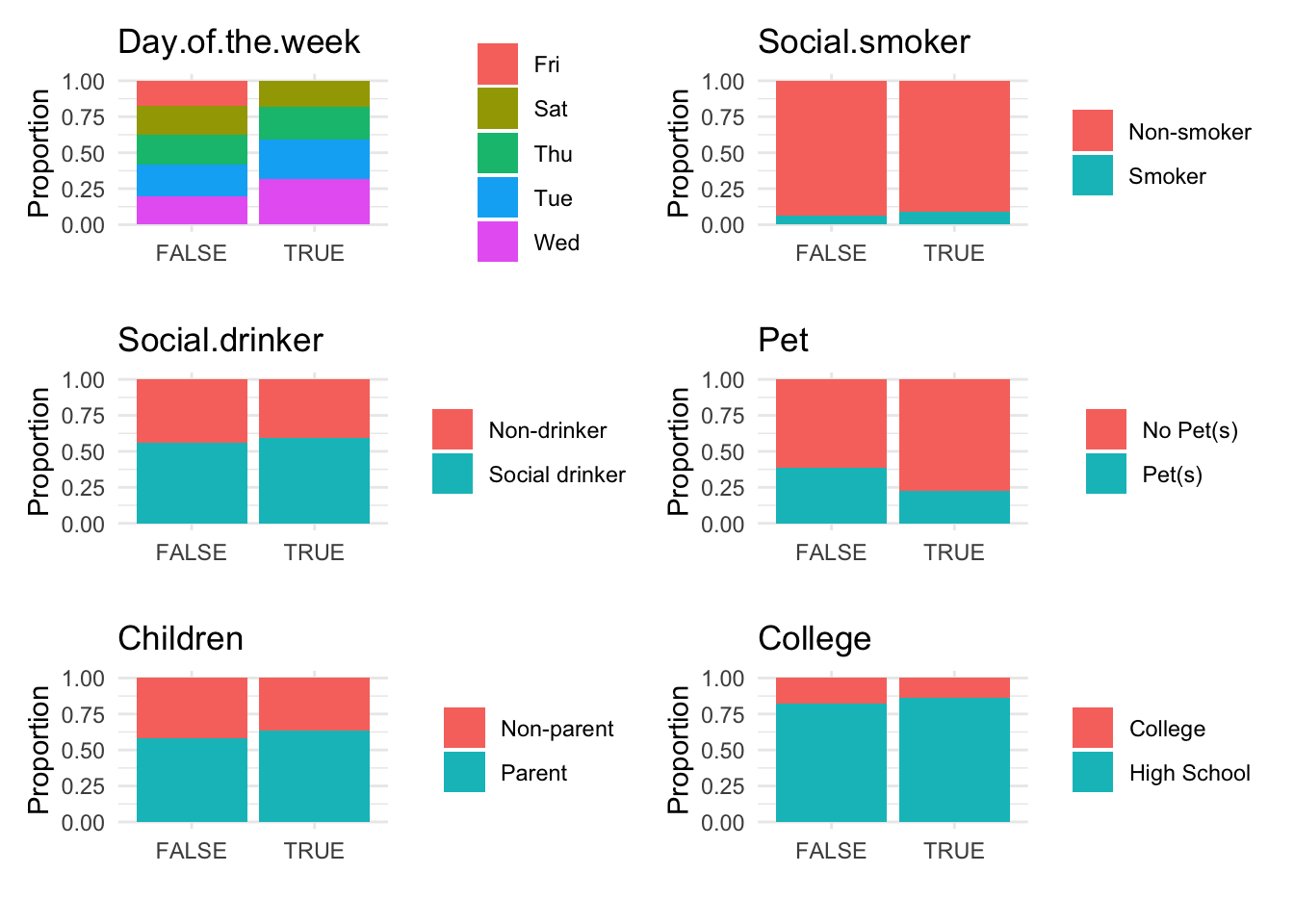
However, upon reviewing these visualizations, we observe that neither the box plots of numeric data nor the bar plots of categorical data show a strong difference between anomalous and non-anomalous observations. This finding suggests that while anomalies are detected, their characteristics might not significantly diverge from the norm based on the analyzed variables.
12.3 Identifying Anomalies Using k-Nearest Neighbors
The k-Nearest Neighbors (k-NN) algorithm is a non-parametric method commonly utilized for classification and regression. However, it can also be effectively adapted for anomaly detection. In this context, the principle is that typical data points are generally located near their neighbors, while anomalies are positioned further away. By calculating the distance to the nearest points, we can identify anomalies as those instances that have a significantly greater average distance to their neighbors compared to normal points. The following are the basic steps to search for anomalous observations Using k-NN.
Step 1: Data Preparation
Breaking down the code
- Dummy Variables Creation: Converts categorical variables into dummy variables.
-
Remove Multicollinearity: The
remove_first_dummy = TRUEoption avoids multicollinearity by removing the first dummy variable. -
Remove Factor Columns: Uses
select(-where(is.factor))to remove all factor columns, ensuring that the dataset consists only of numeric variables necessary for k-NN.
Step 2: k-NN Model Training
Breaking down the code
-
Load Libraries: Loads
caretanddbscanfor modeling and distance calculation. - Set Seed: Ensures that the random processes in the model are reproducible.
- Calculate k: Determines the optimal number of neighbors using a heuristic.
-
Calculate Distances: Uses
kNNdistto compute distances to the k-th nearest neighbor.
Step 3: Anomaly Detection
Breaking down the code:
- Calculate Anomaly Scores: Adds a new column for distances calculated previously.
- Flag Anomalies: Flags data points whose distances are greater than the 95th percentile of all distances as anomalies.
Step 4: Visualizing the results
Visualizing the results can help highlight the anomalies within the data.
# Plotting distances and coloring points based on anomaly status
absenteeism.knn |>
  ggplot(aes(x = 1:nrow(absenteeism), y = distances, color = IsAnomalous)) +
  geom_point() +
scale_color_manual(values = c("black", "red")) 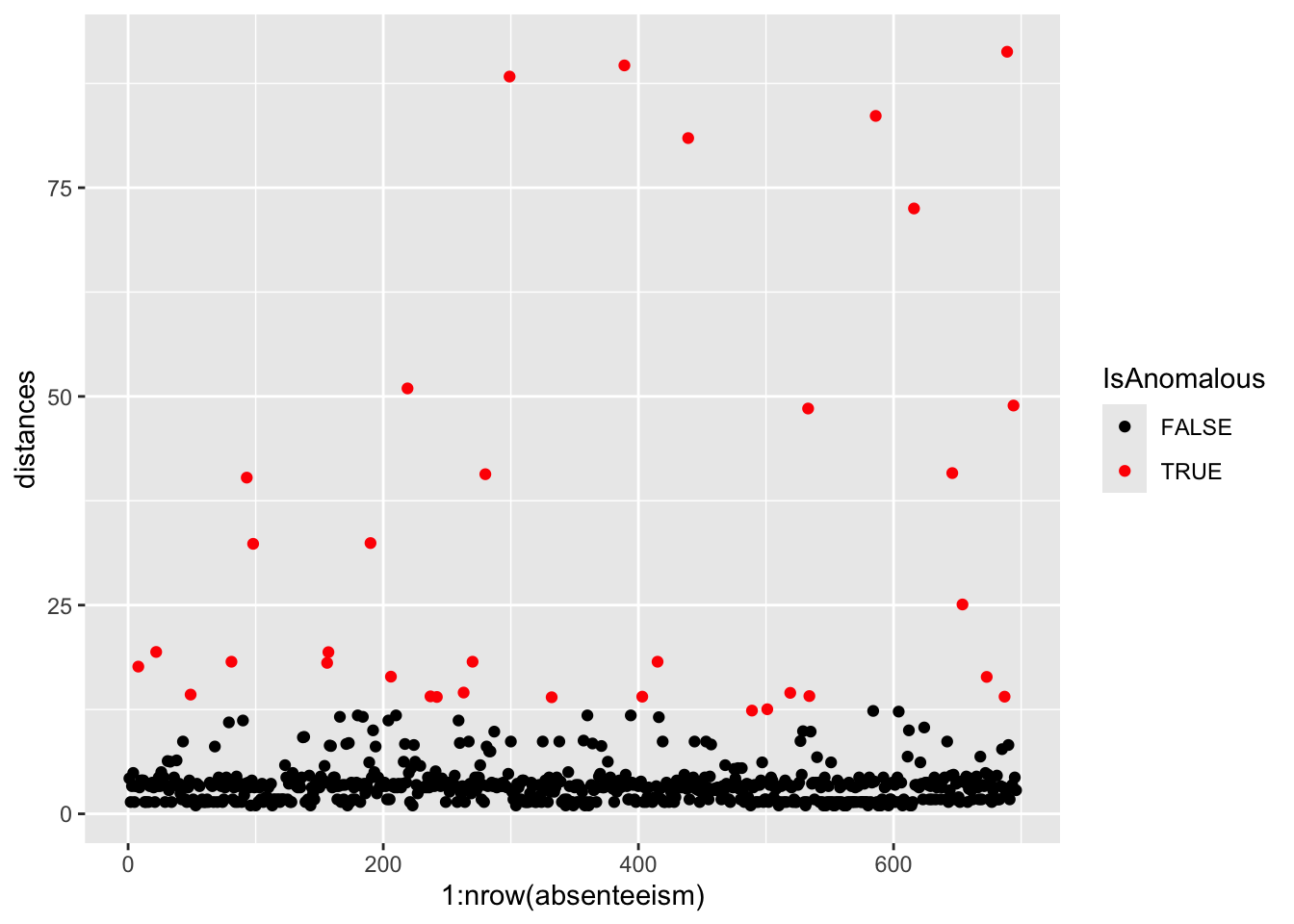
Further analysis of the identified anomalies:
# Removing 'distances' for cleaner data handling
absenteeism.knn <- absenteeism.knn |> select(-distances)

# Visualize anomalies in boxplot and barplot formats
anomaly.boxplot(data = absenteeism.knn, anomaly_indicator = "IsAnomalous") 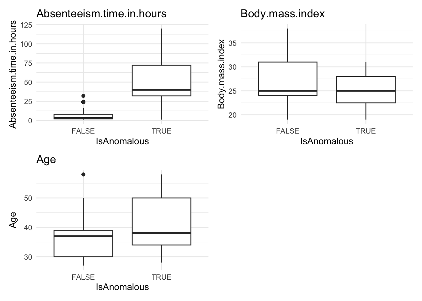
Breaking down the code:
- Visualize with Scatter Plot: Uses ggplot to plot distances and color-code anomalies.
- Data Cleanup: Removes the ‘distances’ column for cleaner data handling.
- Further Visualizations: Implements boxplots and barplots to provide different perspectives on anomalies.
This comprehensive approach not only identifies but also visually represents anomalies, leveraging the k-NN algorithm’s capability to discern deviations based on proximity to neighbors.
Here’s the homework assignment with the addition of example code for each step, using the iris dataset as a guide. This example will help students understand how to apply the instructions to the mtcars dataset.
12.4 Identifying Anomalies Using Random Forest
Random Forest is an advanced ensemble machine learning method that enhances decision tree models. By constructing multiple decision trees from randomly selected subsets of data and features, and aggregating their results, Random Forest effectively reduces the risk of overfitting and is particularly adept at managing datasets with high dimensionality and at performing feature selection.
One key feature of Random Forest in anomaly detection is the proximity matrix, which measures the similarity between pairs of instances. This measurement is based on how often pairs of instances end up in the same terminal nodes (leaf nodes) across the ensemble of trees. The proximity is normalized across all trees, providing a scale from 0 to 1, where higher values indicate greater similarity.
This dataset is ideal for applying Random Forest to identify anomalies, such as atypical patterns of absenteeism that may signal issues like workplace dissatisfaction or health problems.The following are the basic steps for Anomaly Detection Using Random Forest.
Step 1. Data Preparation
Convert categorical variables to dummy variables, removing the first level to avoid multicollinearity, and exclude original factor variables to prepare for modeling.
Breaking down the code
Loading the
fastDummiespackage: This line ensures thatfastDummiesis installed and loaded for use in your R session. If the package isn’t already installed,pacmanwill install it first before loading it.fastDummiesis particularly useful for converting categorical variables into dummy variables.-
Creating dummy variables and preparing the dataset:
-
dummy_cols(remove_first_dummy = TRUE): Converts factor variables in the datasetabsenteeisminto dummy variables, which are binary (0/1) columns that represent the presence or absence of each category in the original factor variables. Theremove_first_dummy = TRUEoption omits the first dummy column to avoid multicollinearity in statistical models. -
select(-where(is.factor)): This command, using thedplyrpackage, removes the original factor columns from the dataset. It selects columns to keep by excluding those that are still factors, cleaning up the dataset post-dummy variable creation.
-
Step 2. Random Forest Model Training
Load the necessary package.
Before training the Random Forest model, it’s crucial to determine the optimal number of trees (ntree). While a larger number of trees generally improves model accuracy and stability, it also increases computational cost and time. The key is to find a balance where adding more trees does not significantly improve model performance. Typically, model performance stabilizes after a certain number of trees, which can be determined through cross-validation or by plotting the model error as a function of the number of trees and observing where the error plateaus.
In this example, we use 500 trees as a starting point, which often provides a good balance for a range of datasets. We enable the proximity option to compute the similarity matrix needed for anomaly detection, which is pivotal in identifying unusual data patterns.
Breaking down the code
set.seed(123): This function is used to set the seed of R’s random number generator, which is useful for ensuring reproducibility of your code. When you set a seed, it initializes the random number generator in a way that it produces the same sequence of “random” numbers each time you run the code. This is particularly important in modeling procedures that involve random processes, such as random forests, because it ensures that you get the same results each time you run the model with the same data and parameters.randomForest(absenteeism.rf, ntree = 500, proximity = TRUE): This line of code is creating a random forest model using therandomForestfunction. Here’s what each parameter means:
-
absenteeism.rf: This is the dataset being used to train the model. Typically, this dataset would be formatted such that each row is an observation and each column is a feature, except for one column which is the response variable (target). Ensure that your dataset is preprocessed appropriately, as the random forest algorithm requires numeric inputs. -
ntree = 500: This parameter specifies the number of trees to grow in the forest. Generally, more trees in the forest can improve the model’s performance but will also increase the computational load. The choice of 500 trees is a balance between performance and computational efficiency. -
proximity = TRUE: When set to TRUE, this parameter tells the function to calculate a proximity matrix that measures the similarity between pairs of cases. If two cases end up in the same terminal nodes frequently, they are considered to be similar. This matrix can be useful for identifying outliers, for imputing missing data, or for reducing the dimensionality of the data.
The randomForest function builds a model that can be used for both classification and regression tasks, depending on the nature of the target variable in your dataset. The model works by constructing multiple decision trees during training and outputting the class that is the mode of the classes (classification) or mean prediction (regression) of the individual trees.
Step 3. Anomaly Detection
Calculate an anomaly score for each instance by inverting the mean proximity value. Instances with scores exceeding the 95th percentile are flagged as anomalies.
Breaking down the code:
Step 1. mutate(score = 1 - apply(rf_model$proximity, 1, mean)): This line adds a new column score to the absenteeism.rf dataset. The score is calculated by taking the mean of each row in the proximity matrix (rf_model$proximity) obtained from the random forest model. The apply function with MARGIN = 1 computes the mean for each row. Subtracting this mean from 1 inverts the proximity values, converting them into anomaly scores. A lower mean proximity suggests greater distance from other instances, hence a higher anomaly score.
Step 2. absenteeism.rf$score > quantile(absenteeism.rf$score, 0.95): This line creates a logical vector that flags each instance as anomalous if its anomaly score is greater than the 95th percentile of all scores. The quantile function is used to find the 95th percentile, and instances exceeding this threshold are considered significant outliers or anomalies.
Step 4. Result Visualization
Visualize the anomaly scores and highlight potential outliers using different colors to differentiate between normal and anomalous instances.
pacman::p_load(ggplot2)
ggplot(absenteeism.rf, aes(x = 1:nrow(absenteeism), y = score)) +
 geom_line() +
 geom_point(aes(color = IsAnomalous), size = 2) +
 scale_color_manual(values = c("black", "red"))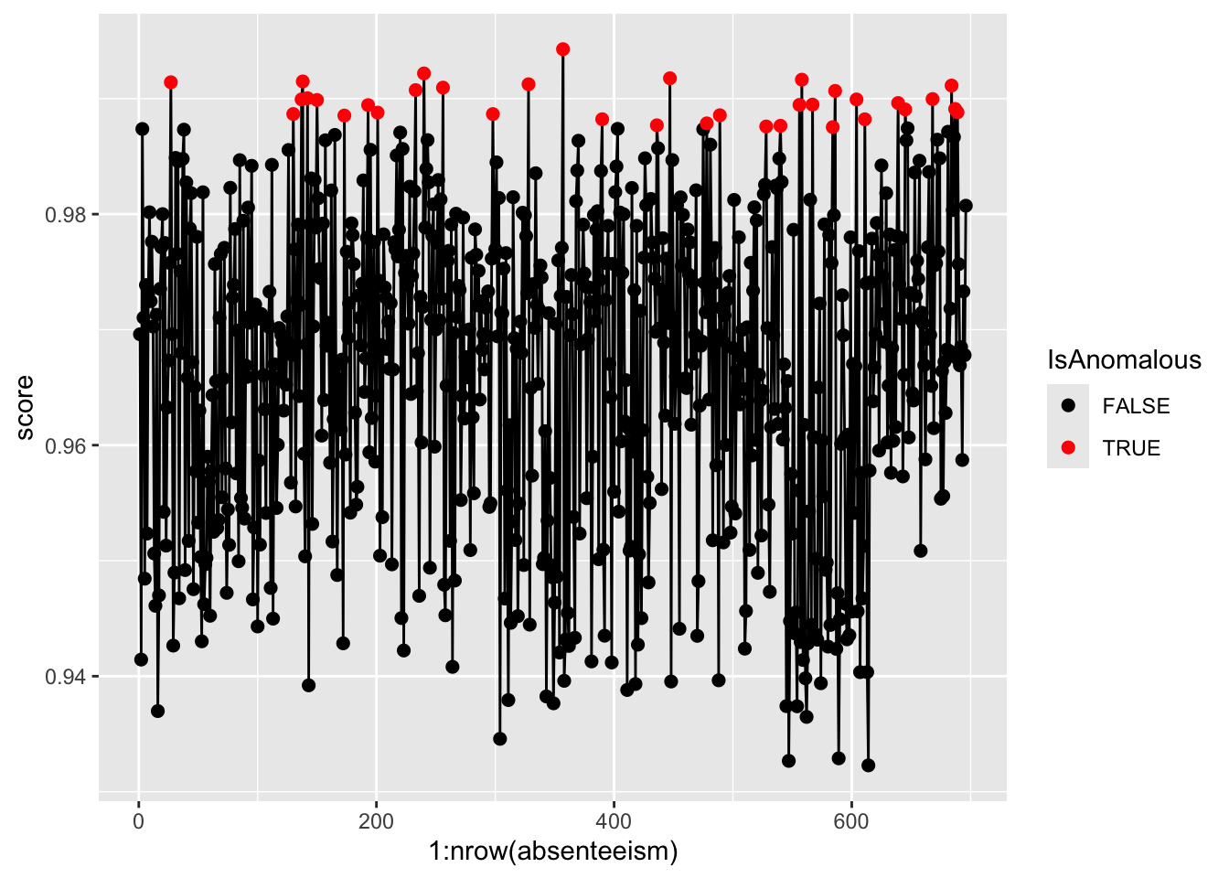
Step 5. Further Analysis with Plots
Analyze the distribution of anomalies using box and bar plots to explore differences in numeric and categorical data between normal and anomalous observations.
absenteeism.rf <- select(absenteeism.rf, -score)
anomaly.boxplot(data = absenteeism.rf, anomaly_indicator = "IsAnomalous")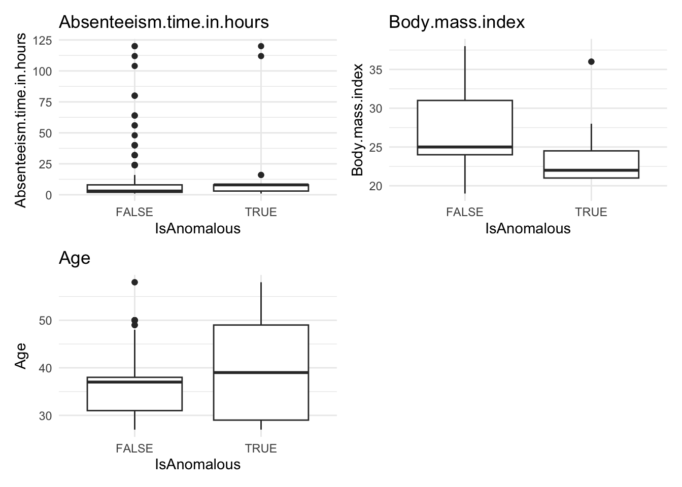
Anomalous observations typically exhibit a lower average BMI, and they have a higher proportion of smokers and pet owners. Other metrics are similar for both anomalous and non-anomalous groups.
12.5 Homework Assignment: Anomaly Detection in Automotive Data
12.5.1 Objective:
Explore anomaly detection techniques using the mtcars dataset to identify unusual observations in automotive specifications. Apply three different statistical methods: linear regression analysis, k-Nearest Neighbors (k-NN), and Random Forest.
12.5.2 Dataset:
The mtcars dataset available in R contains data on 32 automobiles (1973-74 models) with 11 variables such as MPG (miles per gallon), number of cylinders, horsepower, and weight.
12.5.3 Instructions:
Step 1: Setup and Data Loading - Load the necessary R packages. If not installed, install them using the following commands:
Step 2: Data Preparation - Convert categorical variables (if any) to factor variables. In mtcars, convert cyl, vs, am, and gear into factors using the mutate() function from dplyr.
Step 3: Anomaly Detection using Linear Regression - Fit a linear regression model with MPG as the dependent variable and all other variables as predictors.
- Calculate and inspect residuals. Consider observations with residuals greater than 2 standard deviations from the mean as potential outliers.
- Create a diagnostic plot to visualize these outliers.
# Generate the plot of residuals versus fitted values
ggplot(plot_data, aes(x = Fitted, y = Residuals)) +
  geom_hline(yintercept = 0, linetype = "dashed", color = "grey") +
  geom_point(aes(color = Residuals > threshold)) +
  scale_color_manual(values = c("black", "red")) +
  labs(title = "Residual vs. Fitted Plot",
       x = "Fitted Values",
       y = "Residuals",
       color = "Threshold Exceeded") +
  theme_minimal()
Step 4: Anomaly Detection using k-NN
- Use the
kNNdistfunction from thedbscanpackage to calculate the distance to the k-th nearest neighbor. Selectkas the square root of the number of observations.
- Identify anomalies as observations where the distance is greater than the 95th percentile of all distances.
- Visualize these anomalies using a plot of anomaly scores.
ggplot(mtcars.knn, aes(x = row.names(mtcars.knn), y = distances, color = IsAnomalous)) +
  geom_point() +
  scale_color_manual(values = c("black", "red")) +
  theme(axis.text.x = element_text(angle = 45, hjust = 1))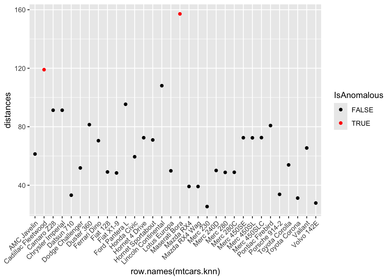
Step 5: Anomaly Detection using Random Forest - Use the randomForest package to fit a model on the dataset, enabling the proximity option to calculate the proximity matrix.
- Derive anomaly scores from the proximity matrix and flag instances with scores above the 95th percentile as anomalies.
- Visualize these anomalies using a plot of anomaly scores.
pacman::p_load(ggplot2)
ggplot(mtcars.rf, aes(x = row.names(mtcars.rf), y = score)) +
 geom_line() +
 geom_point(aes(color = IsAnomalous), size = 2) +
 scale_color_manual(values = c("black", "red")) +
  theme(axis.text.x = element_text(angle = 45, hjust = 1))
`geom_line()`: Each group consists of only one observation.
ℹ Do you need to adjust the group aesthetic?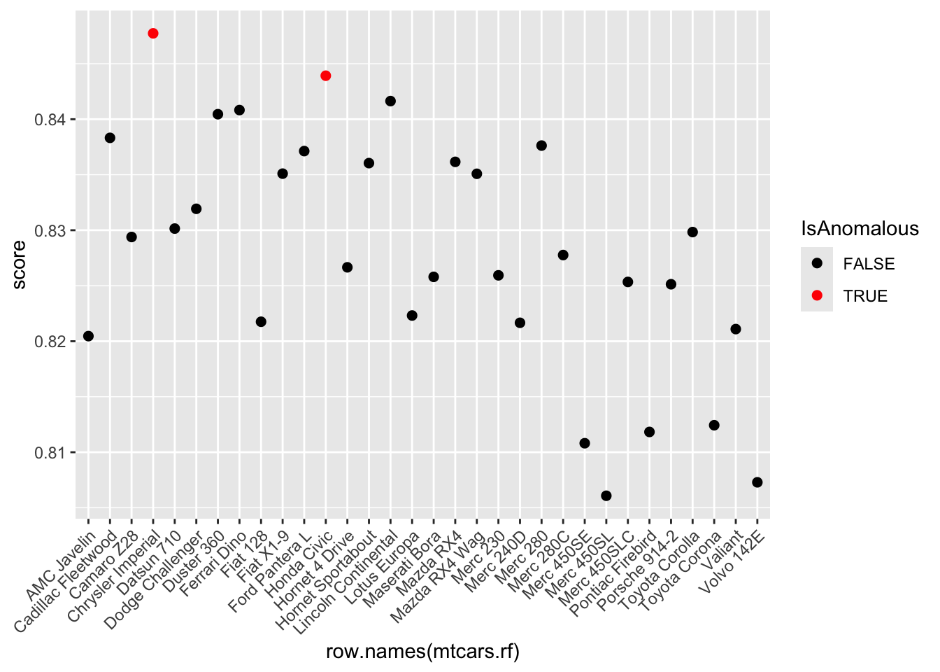
Step 6: Analysis and Comparison - Compare the results from the three methods. Identify which observations are consistently flagged as anomalies across the different techniques. - Provide a brief analysis explaining why these observations might be considered anomalies and discuss the potential implications of these anomalies on automotive performance. Highlight any noticeable differences between anomalous and non-anomalous observations.
Step 7: Report Writing - Compile your findings, including the methodology, results, and detailed discussion, into a structured Quarto document. Incorporate plots to visually support your analysis. - Conclude with your reflections on the effectiveness of each anomaly detection method used in this study.
Submission Requirements: - Students are not required to submit their Quarto document (.qmd file). Instead, render your Quarto document to a Microsoft Word format (.docx) and submit this document. - Ensure that the rendered Word document includes all necessary plots and outputs to comprehensively present your analysis.