Loading required package: pacman5 Data Preparation and Cleaning
5.1 Chapter Goals
Upon concluding this chapter, readers will be equipped with the skills to:
- Understand the principles of tidy data and its importance in data analysis, including the organization of datasets to facilitate easy access and manipulation.
- Utilize the Tidyverse collection of R packages for efficient data import, tidying, manipulation, and visualization, enhancing the data analysis workflow.
- Implement data importing techniques for common file formats such as CSV and Excel, using Tidyverse packages like
readrandreadxl. - Apply
dplyrfunctions for data manipulation tasks, including filtering, selecting, arranging, mutating, and summarizing datasets to extract meaningful insights. - Conduct data tidying operations with
tidyr, transforming datasets between wide and long formats, to adhere to tidy data principles and prepare data for analysis.
5.2 The Essence of Tidy Data
The often-quoted statistic in data analysis is that 80% of the work involves cleaning and preparing the data, a task that is not just a preliminary step but a continuous necessity throughout the analytical process. As new challenges emerge or additional data is gathered, the cycle of cleaning and preparation repeats. This chapter delves into a crucial subset of data cleaning known as data tidying, which is the practice of structuring datasets to streamline analysis.
Data tidying is underpinned by a set of principles that provide a standardized approach to organizing the values within a dataset. Such a standard is invaluable as it simplifies the initial stages of data cleaning, eliminating the need to reinvent procedures for each new dataset. The tidy data paradigm is designed to ease the exploration and analysis of data, as well as the development of analysis tools that are interoperable, reducing the time spent on translating outputs from one tool to input for another. Tidy datasets and tools that adhere to this standard work in tandem, allowing analysts to concentrate on the substantive questions of their domain rather than the logistical hurdles of data manipulation.
5.2.1 Defining Tidy Data
The concept of tidy data draws an analogy to Leo Tolstoy’s observation about families: while every tidy dataset shares common characteristics, each messy dataset is unique in its disorder. Tidy datasets align the dataset’s structure—its physical layout—with its semantics—the meaning of its data. This alignment involves a clear vocabulary for describing data structure and semantics, leading to a definition of tidy data.
5.2.1.1 Data Structure
Statistical datasets are typically structured as data frames, consisting of rows and columns, with columns usually labeled and rows occasionally so. However, the mere description of data in terms of rows and columns is insufficient to capture the essence of a dataset’s structure, as the same data can be organized in various layouts without altering its underlying meaning.
5.2.1.2 Data Semantics
A dataset comprises values, which can be numbers (quantitative) or strings (qualitative), organized by variables and observations. A variable groups all values measuring the same attribute across different units, while an observation aggregates all values from the same unit across various attributes.
5.2.2 Principles of Tidy Data
In the realm of tidy data, the organization of data adheres to three fundamental principles:
Each variable forms a column: This principle ensures that each column in the dataset represents one and only one variable, facilitating easy access to all values associated with a variable.
Each observation forms a row: This ensures that each row in the dataset contains all information pertaining to a single observation, making it easier to analyze or compare individual data points.
Each value occupies a single cell: By adhering to this principle, the dataset maintains a granularity that ensures each cell in the dataset contains only one piece of information, thereby eliminating ambiguity and complexity in data interpretation.
These principles align with Codd’s 3rd normal form, a concept from database design, but are reframed in statistical language and applied to a single dataset rather than to the interconnected datasets typical in relational databases. By contrast, any dataset arrangement that deviates from these principles is considered “messy” data.
The tidy data format not only clarifies the dataset’s semantics but also explicitly defines an observation, aiding in the identification of missing values and their implications. For instance, in a classroom dataset, an absence might be indicated by a missing value, influencing the approach to computing final grades or class averages.
5.2.3 The Advantages of Tidy Data
Tidy data offers a standardized method for mapping a dataset’s meaning to its structure, simplifying the extraction of variables for analysis. This standardization is particularly beneficial in vectorized programming languages like R, where tidy data aligns with the language’s data manipulation and analysis paradigms. Moreover, tidy data facilitates a logical ordering of variables and observations, enhancing readability and easing the identification of variables fixed by design versus those measured during an experiment.
5.3 Introduction to the Tidyverse
The Tidyverse is an ecosystem of R packages designed to facilitate data science tasks with a consistent philosophy, grammar, and data structure. It simplifies the process of data import, cleaning, manipulation, visualization, and analysis. Core packages include ggplot2, dplyr, tidyr, readr, purrr, tibble, stringr, and forcats, each serving a specific function in the data science workflow.
5.3.1 Core Packages Overview
-
dplyr: For data manipulation, offering a set of verbs for data operations. -
ggplot2: For data visualization, based on the Grammar of Graphics. -
tidyr: For data tidying, ensuring a consistent structure. -
readr: For importing data from flat files like CSV and TSV.
5.4 Installing R and the Tidyverse
To streamline package management, use the pacman package. pacman allows for efficient installation and loading of R packages. Install pacman and then use it to install and load the Tidyverse with the following code:
This script checks for pacman and installs it if necessary. It then uses pacman to load the Tidyverse, installing it first if it’s not already installed on your system.
5.5 Data Manipulation with dplyr
dplyr is a cornerstone package within the Tidyverse for data manipulation in R. It introduces several key functions that make data manipulation tasks more intuitive and efficient. Below, we explore these functions using the mtcars dataset, a classic dataset built into R that comprises various aspects of automobile design and performance for 32 automobiles.
dplyr introduces key functions for efficient data manipulation:
-
Filtering:
filter()extracts subsets of rows based on conditions. -
Selecting:
select()focuses on specific columns. -
Arranging:
arrange()reorders rows. -
Mutating:
mutate()adds or modifies columns. -
Summarizing:
summarize()reduces data to summary statistics.
5.5.1 Core Functions and Examples
5.5.1.1 Filtering with filter()
The filter() function extracts subsets of rows from a dataframe based on specified conditions. It’s useful for focusing on observations that meet certain criteria.
Example: Select cars with more than 6 cylinders from the mtcars dataset.
5.5.1.2 Selecting with select()
The select() function allows you to isolate specific columns from a dataframe, simplifying the dataset to only include the information you need.
Example: Choose columns related to car performance, such as miles per gallon (mpg), horsepower (hp), and weight (wt).
5.5.1.3 Arranging with arrange()
arrange() reorders the rows of a dataframe based on the values in one or more columns. It’s helpful for sorting your data in an ascending or descending order.
Example: Order the cars by decreasing horsepower.
5.5.1.4 Mutating with mutate()
The mutate() function is used to add new columns to a dataframe or modify existing ones. This is often done by performing operations on other columns.
Example: Create a new column for car weight in kilograms, assuming 1 lb = 0.453592 kg.
5.5.1.5 Summarizing with summarize()
summarize() reduces your data to summary statistics. This function is particularly powerful when used in conjunction with group_by(), allowing you to compute summaries for groups of data.
Example: Calculate the average miles per gallon across all cars.
Each of these functions plays a vital role in the data manipulation process, enabling you to filter, select, arrange, mutate, and summarize your data efficiently. By integrating these functions into your data analysis workflow, you can enhance the clarity and efficiency of your R programming.
5.5.1.6 Grouping and Summarizing with group_by() and summarize()
While summarize() is great for reducing your entire dataset to summary statistics, its true power is unleashed when combined with group_by(). This pairing allows you to compute summary statistics for distinct groups within your data, making it invaluable for comparative analysis.
Example: Calculate the average miles per gallon (mpg) for each number of cylinders (cyl) in the mtcars dataset.
# Group data by the number of cylinders
average_mpg_by_cyl <- mtcars |>
  group_by(cyl) |>
  summarize(average_mpg = mean(mpg, na.rm = TRUE))

head(average_mpg_by_cyl)
In this example, group_by(cyl) segments the mtcars dataset into groups based on the number of cylinders (cyl). Then, summarize(average_mpg = mean(mpg, na.rm = TRUE)) calculates the average miles per gallon for each group of cylinders. This approach is particularly useful for exploring how certain characteristics (like fuel efficiency in this case) vary across different categories (such as engine size denoted by the number of cylinders).
5.6 Data Tidying with tidyr using Pipe Operator
tidyr is a crucial component of the Tidyverse, designed to facilitate the tidying of data into a format suitable for analysis. The pivot_longer() and pivot_wider() functions are key for reshaping data frames, and their use alongside the pipe operator (|>) significantly improves the readability and efficiency of the code.
5.6.1 Pivoting Longer with pivot_longer()
The pivot_longer() function is adept at transforming data from a wide format, where multiple columns represent different levels of a single variable, into a longer format, where all data for a variable is contained in a single column.
Example with Hypothetical Survey Data: In this example, we’ll work with a fabricated wide-format dataset named survey_data, representing average satisfaction scores for three groups (A, B, and C) over two years (2021 and 2022).
# Hypothetical survey data in a wide format
survey_data <- tibble(
  year = c(2021, 2022),
  A = c(8.2, 8.4),
  B = c(7.8, 7.9)
)
survey_data
# Transforming the wide-format survey data into a longer format
long_survey_data <- survey_data |>
pivot_longer(
cols = -year,
names_to = "Group",
values_to = "Satisfaction_Score"
)
long_survey_dataIn this transformation, pivot_longer() is used to consolidate the six original columns into three: Group, Year, and Satisfaction_Score. The names_sep argument is particularly useful here, as it specifies the character that separates the components of the original column names, allowing tidyr to split these names into separate variables correctly.
# Transforming the long-format data back into a wide format
wide_survey_data_again <- long_survey_data |>
  pivot_wider(
    names_from = c(Group),
    values_from = Satisfaction_Score
  )
wide_survey_data_again
In this transformation, pivot_wider() takes the long_survey_data and spreads the Group values across multiple columns, using Satisfaction_Score as the values to fill the cells. The names_from argument specifies which column in the long-format data will be used to create the new column names in the wide-format data, while values_from specifies which column provides the values. The names_sep argument is used to define a separator that will be inserted between the elements of the new column names, which in this case are derived from the Group and Year columns.
The result, wide_survey_data_again, is a dataframe where each satisfaction score is associated with a specific group and year, similar to the original survey_data but potentially reordered or reformatted based on the transformations applied during the pivot processes.
5.7 Joining Data Sets with dplyr
Combining information from different sources is a common task in data analysis. dplyr offers a variety of join functions to facilitate this, each tailored to different joining scenarios. dplyr offers several join functions:
-
inner_join(): Returns rows with matching values in both datasets. -
left_join(): Returns all rows from the left dataset, with matching rows from the right dataset. -
right_join(): Returns all rows from the right dataset, with matching rows from the left dataset. -
full_join(): Returns all rows from both datasets, with matches where available. -
semi_join(): Returns all rows from the left dataset where there are matching values in the right dataset, but only columns from the left dataset. -
anti_join(): Returns all rows from the left dataset where there are no matching values in the right dataset, keeping only columns from the left dataset.
5.7.1 Preparing Sample Data Frames
Before discussing the various join functions available in dplyr for combining datasets, let’s set up two sample data frames, mtcars1 and mtcars2, to use as examples. These data frames will be subsets of the built-in mtcars dataset in R, with some modifications to illustrate different joining scenarios.
5.7.1.1 mtcars1 DataFrame
This data frame will include a subset of the original mtcars columns, such as mpg, cyl, disp, and hp, along with a new column car_model as a unique identifier.
5.7.1.2 mtcars2 DataFrame
This data frame will contain a different subset of columns, namely gear and carb, along with the car_model column. It will include some car models not present in mtcars1 and exclude others that are, to demonstrate various join behaviors.
mtcars2 <- mtcars[10:25, c("gear", "carb")]
mtcars2$car_model <- rownames(mtcars[10:25, ])
mtcars2$df.2 <- "mtcars2"
mtcars2
With these sample data frames, we can explore how different dplyr join functions operate.
5.7.2 inner_join()
Purpose: Merges rows with matching values in both tables, providing a dataset that includes only the rows common to both tables.
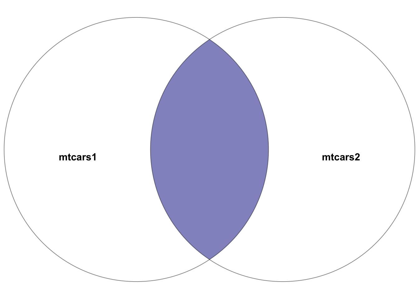
mtcars1 and mtcars2. The highlighted section depicts the result of the inner join–the intersection of the two datasets. In other words, the rows with matching entries in the key columns of both datasets
Example:
# Inner join between mtcars1 and mtcars2 on car_model
joined_data_inner <- inner_join(mtcars1, mtcars2, by = "car_model")
joined_data_inner
This join results in a dataset containing cars present in both mtcars1 and mtcars2, with all columns from both datasets included for the matching rows.
5.7.3 left_join()
Purpose: Returns all rows from the left table (first specified), along with the matching rows from the right table. Rows in the left table without matches in the right table will have NA in the columns from the right table.
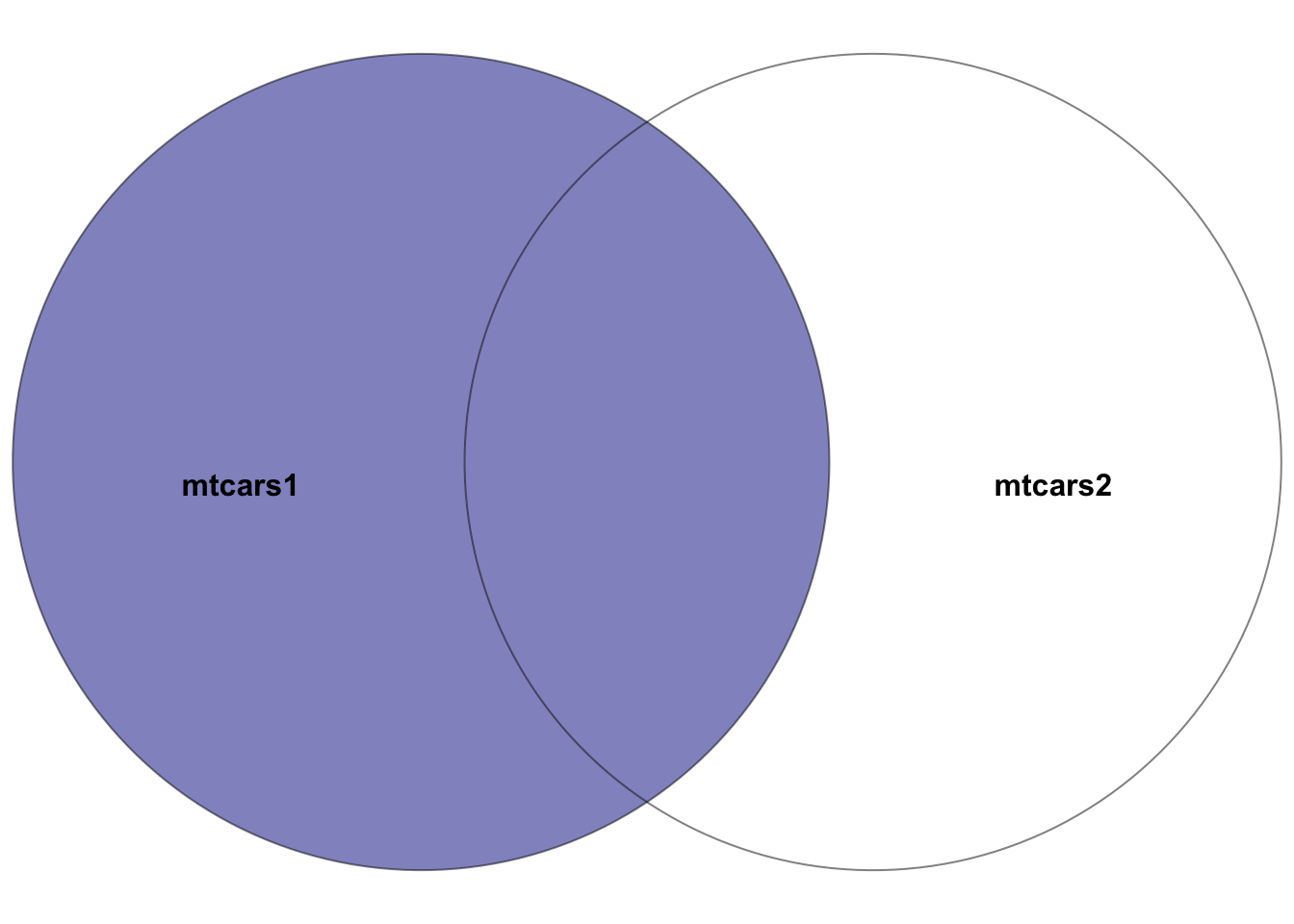
mtcars1 and mtcars2, where the left dataset is mtcars1. The highlighted section depicts the result of the left join–all rows in the left dataset mtcars1 plus the intersection of the two datasets. In other words, the rows with matching entries in the key columns of both datasets
Example:
# Left join mtcars1 with mtcars2 on car_model
joined_data_left <- left_join(mtcars1, mtcars2, by = "car_model")
joined_data_left
This join produces a dataset with all cars from mtcars1, supplemented with gear and carb data from mtcars2 where available.
5.7.4 right_join()
Purpose: Returns all rows from the right table, with matching rows from the left table. Rows in the right table without matches in the left table will have NA in the columns from the left table.
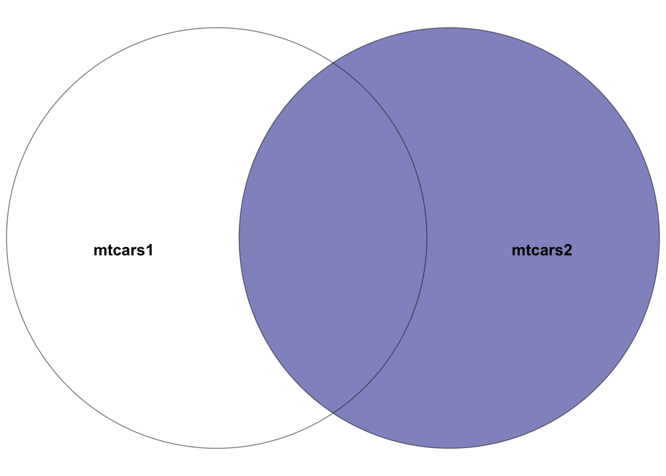
mtcars1 and mtcars2, where the right dataset is mtcars2. The highlighted section depicts the result of the right join–all rows in the right dataset mtcars2 plus the intersection of the two datasets. In other words, the rows with matching entries in the key columns of both datasets
Example:
# Right join mtcars1 with mtcars2 on car_model
joined_data_right <- right_join(mtcars1, mtcars2, by = "car_model")
joined_data_right
This join yields a dataset containing all cars from mtcars2, with mpg, cyl, disp, and hp data from mtcars1 where matches are found.
5.7.5 full_join()
Purpose: Combines all rows from both tables, with matches where available. Rows without matches in the opposite table will have NA in the corresponding columns.
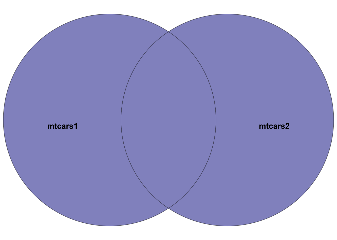
mtcars1 and mtcars2. The highlighted section depicts the result of the full join–all rows in both datasets. Rows in the intersection of the two datasets will have entries in all columns. Rows not in both datasets will have NA’s in missing columns.
Example:
# Full join between mtcars1 and mtcars2 on car_model
joined_data_full <- full_join(mtcars1, mtcars2, by = "car_model")
joined_data_full
This join results in a dataset that includes all cars from both mtcars1 and mtcars2, ensuring no data is lost, and filling missing values with NA.
5.7.6 semi_join()
Purpose: Returns all rows from the left table where there are matching values in the right table, but only includes columns from the left table.
Example:
# Semi join mtcars1 with mtcars2 on car_model
joined_data_semi <- semi_join(mtcars1, mtcars2, by = "car_model")
joined_data_semi
This join creates a dataset with rows from mtcars1 that have a corresponding match in mtcars2, but only retains columns from mtcars1.
5.7.7 anti_join()
Purpose: Returns all rows from the left table where there are no matching values in the right table, keeping only columns from the left table.
Example:
This join produces a dataset consisting of cars in mtcars1 that do not have a match in mtcars2, with columns only from mtcars1.
5.7.8 Considerations
- Be mindful of data duplication, particularly when key columns contain non-unique values.
- Ensure that key columns used for joining have matching data types in both tables.
- Resolve column name conflicts;
dplyrwill append suffixes to duplicate column names to distinguish them.
5.8 Data Cleaning Techniques
Before diving into data cleaning techniques, let’s create a sample DataFrame that contains both missing and duplicate observations to illustrate the process more concretely.
5.8.1 Creating a Sample DataFrame
We can create a sample DataFrame in R with the following characteristics:
- Some rows have missing values (
NA) in one or more columns. - Some rows are duplicates, meaning they are identical across all columns.
# Creating a sample DataFrame with missing values and duplicates
set.seed(123)  # For reproducibility
sensor_data <- data.frame(
  timestamp = seq(as.POSIXct("2024-01-01"), by = "hour", length.out = 20),
  temperature = rnorm(20, mean = 20, sd = 5),
  humidity = rnorm(20, mean = 50, sd = 10)
)

# Introducing missing values randomly
sensor_data[sample(1:20, 5), "temperature"] <- NA
sensor_data[sample(1:20, 5), "humidity"] <- NA

# Adding duplicate rows
sensor_data <- rbind(sensor_data, sensor_data[sample(1:20, 5), ])


sensor_data
In this sample sensor_data DataFrame, we have temperature and humidity readings taken hourly. We introduce missing values in both columns and add some duplicate rows to simulate a realistic dataset that needs cleaning.
5.8.2 Handling Missing Values
Managing missing values is a crucial step in data cleaning. The strategies for handling missing data include removal and imputation.
5.8.2.1 Removing Rows with Missing Values
To clean the dataset, rows with missing values can be removed if losing some data does not significantly impact the analysis.
Here, drop_na() is used on sensor_data to eliminate any row that contains at least one NA value, simplifying subsequent analyses but potentially losing valuable information.
5.8.2.2 Replacing Missing Values
Alternatively, missing values can be replaced with a specific value like the mean or median, which helps maintain the dataset size.
# Replacing missing values with the mean
mean_temp <- mean(sensor_data$temperature, na.rm = TRUE)
sensor_data_clean <- sensor_data |>
  mutate(
    temperature_mean = ifelse(is.na(temperature),mean_temp,temperature)
  )
sensor_data_clean
In this case, missing temperature values are replaced with the column’s mean temperature, computed while ignoring NAs with na.rm = TRUE.
5.8.3 Dealing with Duplicates
Duplicate observations can bias the analysis, making it essential to remove them to maintain data integrity.
5.8.3.1 Removing Duplicate Rows
Removing duplicates ensures that each observation uniquely contributes to the analysis.
# Removing duplicate rows to retain only unique observations
sensor_data_unique <- distinct(sensor_data)
sensor_data_unique
Using distinct(), we remove duplicate rows from sensor_data, keeping only the first instance of each duplicate by default, thus ensuring data uniqueness.
By addressing both missing values and duplicates as demonstrated, we can enhance the quality and reliability of our data analyses.